Technology, Automation, AI, and Labor Market
Learning Objectives
By the end of Week 11, students should be able to:
distinguish automation, augmentation, new-task creation, and organizational redesign as separate channels of technological change;
explain why technology affects labor supply, labor demand, and market-level equilibrium at the same time;
use a task-based framework to organize historical ICT, robot, and contemporary AI evidence;
separate direct displacement from indirect productivity, reinstatement, and reallocation effects;
distinguish tasks from occupations, exposure from adoption, and within-firm effects from local-labor-market equilibrium effects;
evaluate worker adjustment through learning, retraining, occupational switching, and skill obsolescence;
interpret empirical designs by naming the identifying variation, unit of observation, observed margin, and key equilibrium margin left offstage;
connect Week 10 aggregate adjustment to Week 11 structural adjustment and bridge forward to Week 12 trade and offshoring.
Opening Orientation
The economic question for Week 11 is explicit: how do technology, automation, and AI reshape work through worker adaptation, firm labor demand, and market-level reallocation?
Bridge
Week 10 studied cyclical adjustment. The core objects were unemployment, vacancies, separations, job-to-job mobility, wages, and match quality. Week 11 keeps those labor-market objects onstage but changes the shock. Instead of a business-cycle disturbance, the shock now comes from technology adoption, automation, software, robots, and AI. The lecture therefore remains a labor-economics week rather than drifting into a general technology survey.
The first discipline for the week is to organize technology around three linked objects.
Supply-side adjustment: worker learning, retraining, search/application technology, occupational switching, and skill obsolescence.
Demand-side adjustment: task substitution, task complementarity, automation, augmentation, hiring redesign, and within-firm labor demand.
Market-level adjustment: local labor-market reallocation, wage and employment incidence, labor-share changes, concentration, and cross-place equilibrium spillovers.
Table 1:Technology margins map for Week 11
| Technology type | Typical supply-side channel | Typical demand-side channel | Typical market-level channel | Canonical empirical objects |
|---|---|---|---|---|
| ICT / software | skill updating, task reorganization, occupational switching | complementarity with educated labor, middle-skill task substitution | polarization, occupational restructuring | occupation/industry employment shares, wage premia, task content |
| Industrial robots | retraining, reassignment, exits from exposed sectors | direct substitution in routine/manual tasks | local reallocation, service offsets, wage incidence | commuting-zone or region exposure, worker transitions, sectoral adjustment |
| AI prediction/classification tools | changed application/search and screening processes; learning support | altered hiring mix, non-AI hiring crowd-out, task substitution in cognitive work | occupational exposure gradients, firm concentration, reallocation | vacancies, skills, adoption indicators, matched firm data |
| Generative AI / copilot tools | faster learning, lower onboarding costs, changed worker progression | productivity scaling, differential effects by worker experience, reallocation of supervision | wage compression or dispersion, organizational redesign, new tasks | field experiments, worker productivity logs, firm adoption, occupation exposure |
| General purpose technologies / broad innovation waves | education and training responses, long-run skill accumulation | productivity growth, new task creation, labor-share changes | long-run demand shifts across occupations and regions | historical text/patent measures, census occupations, long-run wages/employment |
Table Table 1 is the opening map for the week. It keeps the lecture centered on labor-market margins rather than collapsing robots, ICT, and AI into one undifferentiated shock.
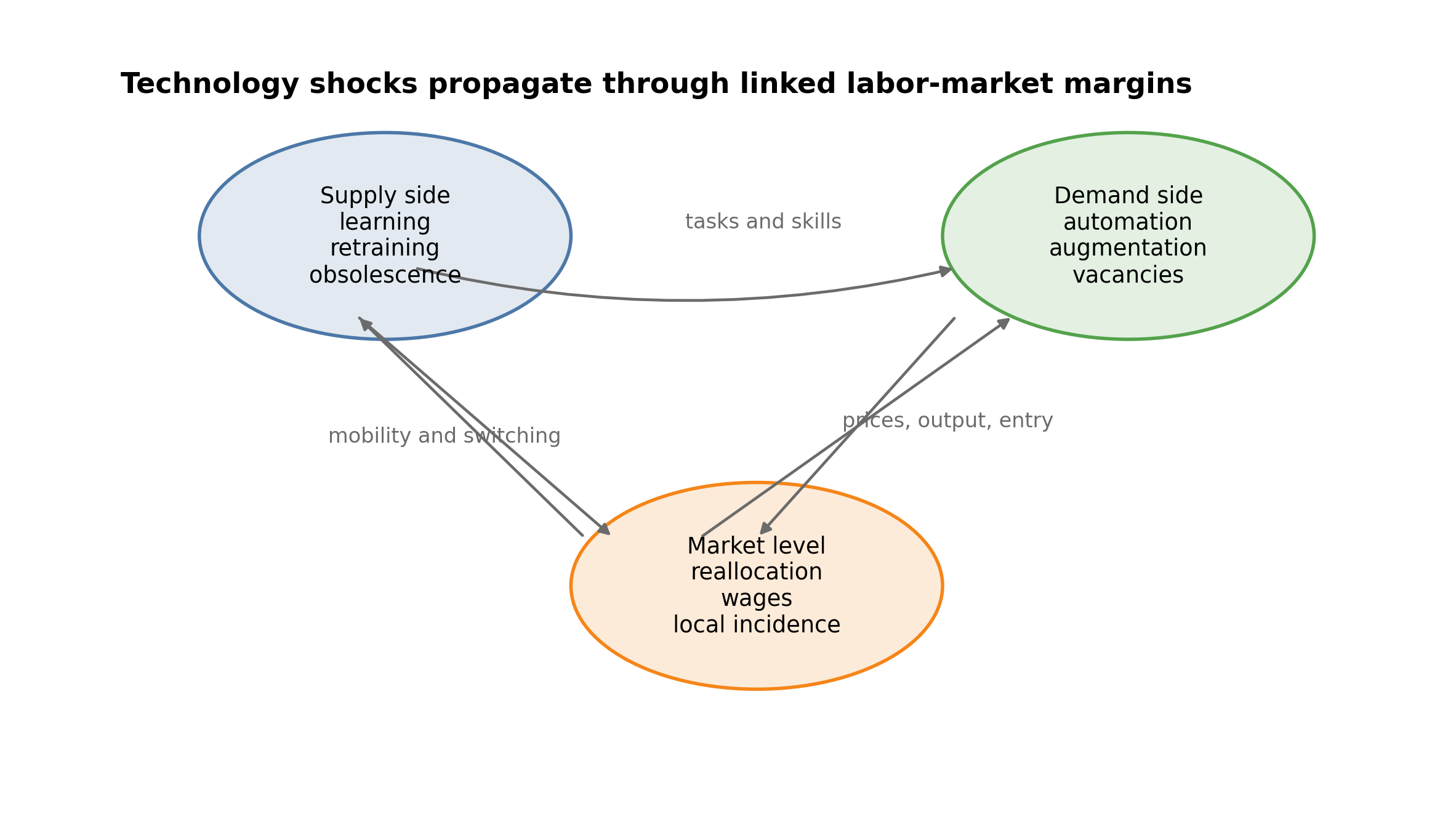
Figure 1:Week 11 links worker adaptation, firm-side labor demand, and market-level equilibrium. The same technology can change all three margins at once, so neither pure labor-demand language nor pure “AI future of work” language is enough.
Figure Figure 1 previews the lecture structure. The important move is to treat technology as a shock that propagates through feedback loops rather than only through a single firm labor-demand curve.
Field Core
Technology as a labor-market shock
It helps to classify technologies before classifying effects. The relevant categories for Labor II are ICT and software, industrial robots, prediction/classification systems, generative AI tools, and broader general-purpose technologies Autor, 2015Autor, 2022. These technologies differ in capital embodiment, diffusion speed, observability, and which margins are directly measurable, but they share one labor-economics feature: they change the mapping from tasks to workers, firms, and markets.
The same technology can generate displacement, augmentation, output expansion, new tasks, and organizational redesign at the same time Acemoglu & Restrepo, 2019. That is why this week must keep explicit distinctions in view.
Tasks are units of activity; occupations are bundles of tasks.
Exposure is a predicted susceptibility measure; adoption is realized technology use.
Within-firm evidence captures partial-equilibrium labor-demand responses more cleanly than market-level equilibrium incidence.
Historical ICT and robot evidence should not be read as if it were already evidence about very recent AI.
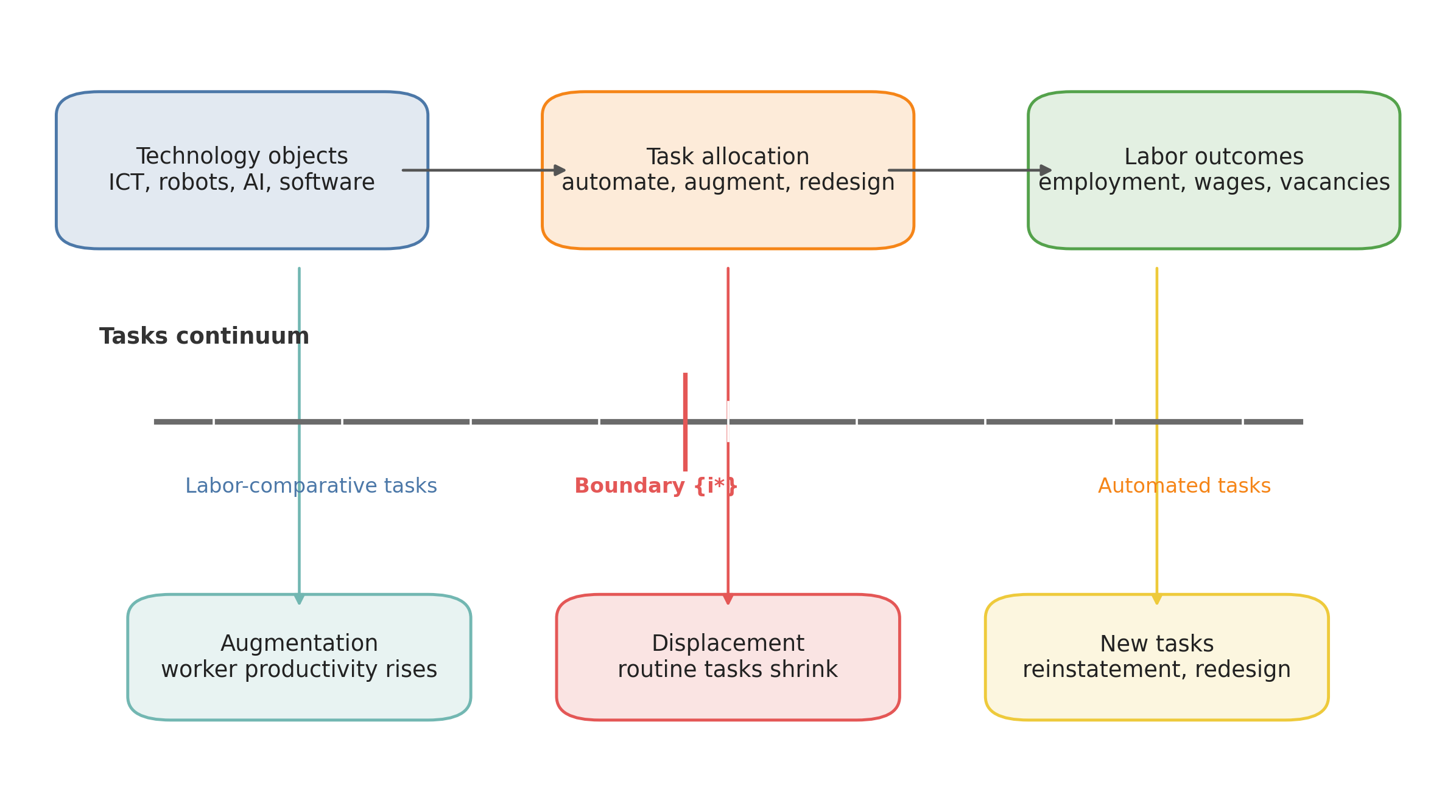
Figure 2:A task-based framework turns technology into a labor-market mapping problem. Technologies shift the boundary between tasks done by workers, tasks automated by capital or software, and tasks newly created or reorganized inside firms.
Figure Figure 2 is the conceptual anchor. Labor outcomes depend on which tasks move across the automation boundary, which tasks become more productive when paired with workers, and which tasks are newly created.
Formal core: tasks, automation boundaries, and worker adjustment
The smallest aggregate task-based production object is
where task contributes to final output and governs substitution across tasks Acemoglu & Autor, 2011. This object is useful because it makes technological change a statement about task productivity, task assignment, and the elasticity with which firms can reorganize activity across tasks.
Let labor complete task with unit cost and capital, robots, or AI systems complete task with unit cost . Then the automation boundary solves
Equation (2) is the task-allocation object for the week. A fall in technology cost or a rise in machine productivity expands the set of automated tasks , but that does not by itself tell us whether total labor demand rises or falls. That depends on productivity gains, output expansion, and whether new tasks or complementary tasks appear elsewhere in the system Acemoglu & Restrepo, 2019.
The lecture therefore needs a decomposition that separates direct displacement from indirect offsets:
Equation (3) is deliberately schematic. It does not claim those terms are directly observed in every paper. It clarifies the empirical question students should ask whenever they see a technology coefficient: which part looks like direct substitution, which part looks like output expansion, and which part looks like new-task or reinstatement effects?
Supply-side adjustment belongs in the formal core too. Let worker human capital evolve according to
where is new investment in skills and is technology-dependent obsolescence. Rapid technical change raises for some workers and lowers the value of old experience even when it raises productivity for others Bartel & Sicherman, 1998Deming & Noray, 2020. This is the supply-side object that keeps skill acquisition and skill obsolescence in the same frame.
The reduced-form exposure equation that organizes much of the empirical literature is
where may be a commuting zone, occupation, industry, firm, or worker-time cell. Equation (5) is intentionally broad because the literature uses different units. The crucial question is whether measures predicted exposure or realized adoption, and whether is a demand-side, supply-side, or market-level outcome.
Historical perspective: why labor demand did not simply disappear
The long-run perspective matters because fears of labor-saving technology predate AI by centuries. Autor’s central argument is that aggregate labor demand did not collapse because automation eliminated some tasks while raising demand for other tasks, new goods, and complementary capabilities Autor, 2015. Acemoglu and Restrepo formalize the same point with displacement and reinstatement: automation can reduce demand for labor in automated tasks even as new tasks later pull labor back into production Acemoglu & Restrepo, 2019.
The historical lesson is not that technology is always benign. It is that labor-market effects are mediated by task structure, product demand, institutions, and the speed of worker adjustment. Acemoglu and Autor’s task framework turned this into a precise distinction between occupations and the tasks inside them Acemoglu & Autor, 2011. Michaels, Natraj, and Van Reenen then show how ICT adoption was associated with rising demand for high-skill tasks and declining routine middle-skill work across countries Michaels et al., 2014.
Table 2:Evidence by margin and era for technology and labor
| Margin | Historical / long-run evidence | Robot / automation era evidence | Contemporary AI evidence | What students should compare |
|---|---|---|---|---|
| Employment levels | Autor, 2015, Michaels et al., 2014 | Acemoglu & Restrepo, 2020, Dauth et al., 2021 | Aghion et al., 2025, Acemoglu et al., 2020 | direct displacement vs output expansion vs reallocation |
| Wage and labor-share effects | Acemoglu & Restrepo, 2019, Autor, 2022 | Acemoglu & Restrepo, 2020, Graetz & Michaels, 2018 | still emerging; use Brynjolfsson et al., 2025 and Aghion et al., 2025 cautiously | who gains, who loses, and which object is actually observed |
| Task / occupational composition | Acemoglu & Autor, 2011, Michaels et al., 2014 | Dauth et al., 2021 | Felten et al., 2018, Acemoglu et al., 2020 | tasks vs occupations, exposure vs realized change |
| Worker adaptation / learning | Bartel & Sicherman, 1998 | indirect and slower-moving in robot papers | Deming & Noray, 2020, Brynjolfsson et al., 2025 | skill obsolescence, training, experience gradients |
| Global / comparative perspective | cross-country ICT polarization | 17-country robot evidence and Germany | France firm-level AI adoption, other new country studies as extension | institutions, equilibrium offsets, and why external validity is hard |
Table Table 2 keeps the historical, robot, and AI eras comparable by margin rather than by hype cycle. That is a better discipline than treating all technology episodes as identical.
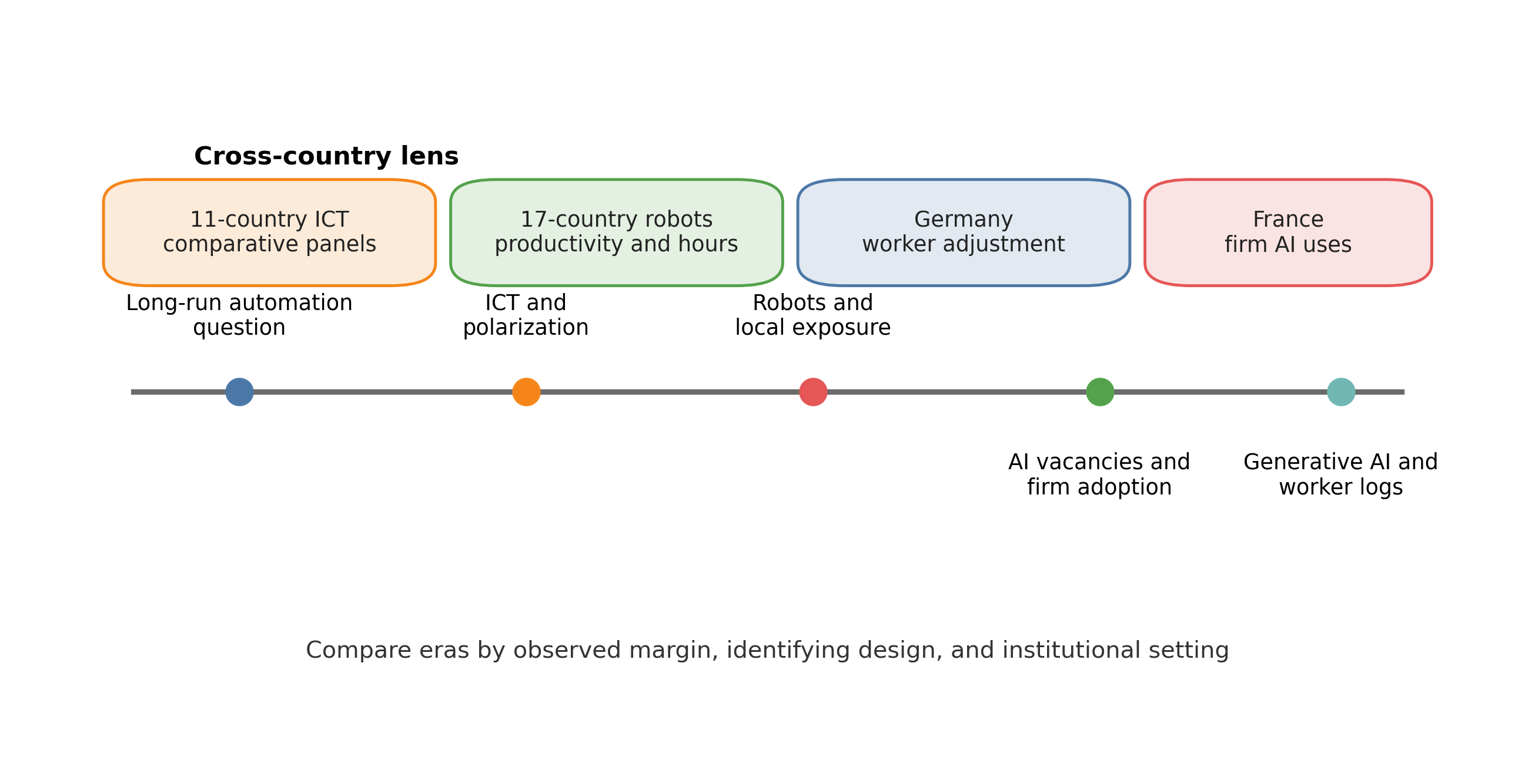
Figure 3:Historical and global evidence should be read as a sequence of technology waves, design choices, and institutional environments. The relevant comparison is not “old technology versus AI” in the abstract, but which margins are observed in each era and setting.
Demand-side evidence: robots, ICT, AI adoption, and vacancies
Demand-side evidence asks how technology changes hiring, employment, occupational mix, wage bills, and vacancy content inside firms and across local labor markets. The most important discipline is to distinguish direct substitution inside exposed tasks from equilibrium effects operating through productivity, output, entry, and reallocation.
Acemoglu and Restrepo’s robot paper uses differential industry robot adoption mapped into local labor-market exposure across U.S. commuting zones Acemoglu & Restrepo, 2020. The identifying variation is shift-share exposure. The unit of observation is the commuting-zone-by-period cell. The observed margins are employment-to-population ratios and wages. The key offstage equilibrium margin is broader national product-demand and price adjustment, which the local design does not fully recover. This is the canonical market-level displacement benchmark.
Graetz and Michaels study industrial robots in a seventeen-country industry panel Graetz & Michaels, 2018. Their identifying variation comes from cross-country, cross-industry robot penetration over time. The unit is industry-country-year. The observed margins are productivity, hours, and wage-bill components. The offstage margin is worker-level reallocation inside countries. The design is strongest for comparative broad patterns, not for within-market worker transitions.
Contemporary AI evidence often sits closer to the firm and vacancy margin. Acemoglu, Autor, Hazell, and Restrepo use online vacancies to measure how AI exposure maps into hiring intentions and skill demand Acemoglu et al., 2020. The identifying variation comes from exposure across occupations and local labor markets. The unit is a vacancy or posting cell. The observed margin is job requirements and vacancy content, not realized employment. That distinction matters because postings tell us what firms seek, not whether staffing or wages ultimately change.
Worker adaptation and labor supply: learning, obsolescence, and search
Week 11 should not treat worker adjustment as a side note. Bartel and Sicherman show that technological change increases the return to skill acquisition and can alter training patterns for young workers Bartel & Sicherman, 1998. The identifying variation in that literature comes from industry or workplace technological change. The unit is typically the worker or worker-job match. The observed margins are training or earnings trajectories. The offstage margin is the longer-run general-equilibrium diffusion of the technology itself.
Deming and Noray make the obsolescence margin concrete by showing that workers in fast-changing STEM occupations experience steep early-career rewards but faster depreciation of accumulated job-specific knowledge Deming & Noray, 2020. The unit is the worker-career spell. The observed margin is earnings dynamics by occupational technological intensity. The key distinction is between skill acquisition and skill obsolescence: the same environment can raise the payoff to learning and shorten the half-life of old expertise at the same time.
Generative AI sharpens the supply-side question because it may change onboarding, supervision, and who can perform high-value tasks soon after entry. Brynjolfsson, Li, and Raymond study worker productivity under generative AI assistance Brynjolfsson et al., 2025. The identifying variation comes from tool access inside a firm setting. The unit is worker-task or worker-shift output. The observed margin is productivity, especially heterogeneity by prior experience. The offstage margin is market-level wage incidence and longer-run job redesign. This is why worker productivity is not the same object as worker welfare.
AI may also change labor supply through application and search technology, but that literature is still thinner than the displacement and vacancy literature. That should be stated plainly. The frontier question is whether AI-assisted job search improves matching quality, changes search intensity, or simply redistributes who wins search tournaments.
Market-level equilibrium and distribution: reallocation, incidence, and labor share
Once supply and demand interact, technology becomes a market-level incidence problem. Acemoglu and Restrepo’s local robot design is again helpful because it captures wage and employment incidence across places rather than only inside firms Acemoglu & Restrepo, 2020. Dauth, Findeisen, Suedekum, and Woessner show that the German response to robots combined manufacturing losses with offsets elsewhere in the economy, making reallocation central to the interpretation Dauth et al., 2021. The identifying variation is again exposure, but the institutional environment differs and so does the equilibrium adjustment path.
This is also where labor-share and inequality questions belong. Technology can raise productivity and still worsen labor-market outcomes for some groups if rents shift toward capital, superstar firms, or already-advantaged workers Autor, 2022. The relevant distinctions are direct displacement versus indirect output effects, and average productivity versus distributional incidence. A productivity gain observed at the firm level does not by itself tell us who captures the surplus.
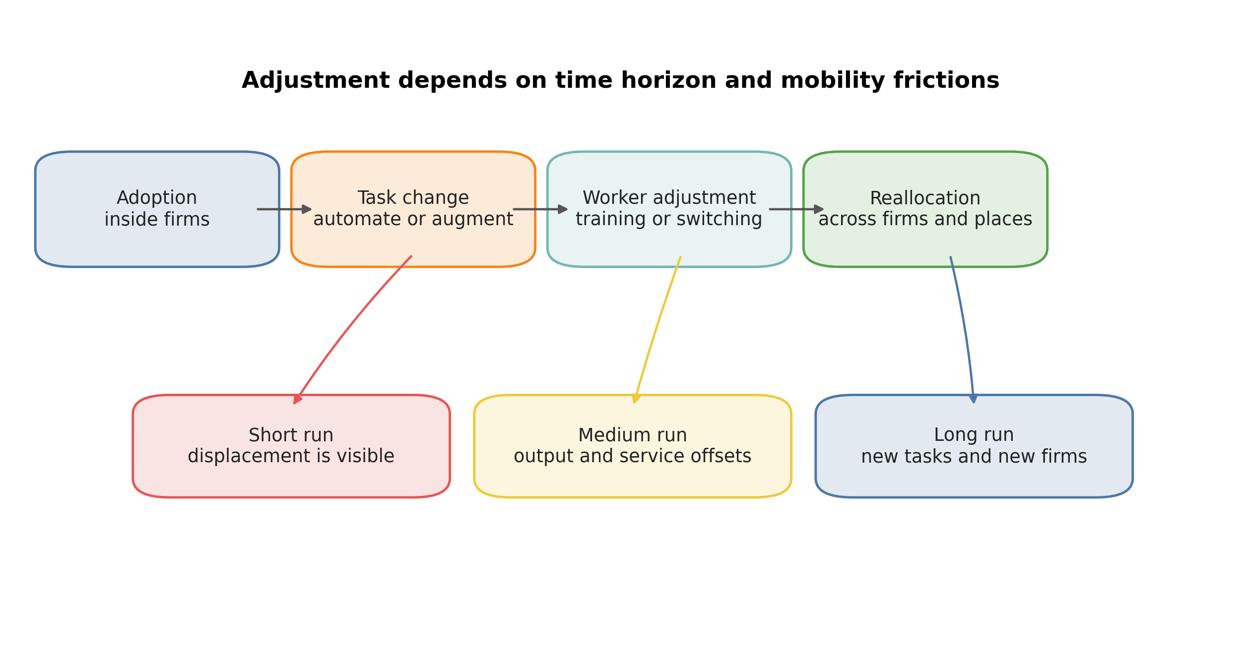
Figure 4:Technology shocks propagate from task reallocation inside firms to retraining, mobility, and local-market incidence. The longer-run outcome depends on output expansion, sectoral offsets, and how quickly workers and places can adjust.
Figure Figure 4 is the week’s equilibrium reminder. Displacement is often the most visible short-run effect, but service offsets, occupational restructuring, and worker mobility determine medium-run incidence.
Contemporary AI evidence: exposure, adoption, and realized labor demand
Recent AI evidence is distinctive because measurement has moved faster than long-run outcome data. Felten, Raj, and Seamans create an occupation-level AI exposure metric by mapping AI capabilities to occupational abilities Felten et al., 2018. The identifying object is descriptive exposure, not treatment. The unit is the occupation. The observed margin is predicted susceptibility. The offstage margin is actual firm adoption and realized worker impact. Exposure measures are useful, but they are not outcomes.
Aghion et al. provide a cleaner adoption-based benchmark by distinguishing different uses of AI in French firms Aghion et al., 2025. The identifying variation comes from realized adoption categories rather than exposure alone. The unit is the firm. The observed margins are labor-demand responses such as employment growth, vacancies, and workforce composition. The key labor insight is that different uses of the same general technology can have different demand effects: automation-style uses can crowd out some hiring while augmentation or complementary uses can expand it.
Labaschin et al. push the measurement frontier by extending exposure ideas from occupations to firms Labaschin et al., 2025. This helps bridge the gap between public task-based exposure measures and actual firm organization, but it still does not eliminate the selection problem in adoption. Firms choose technologies endogenously, and the most adoption-rich data are often the least publicly reproducible.
AI data and measurement: what each source can and cannot identify
Table 3:Data, design, and research-opportunities map for Week 11
| Data / design family | What it measures well | Main limitation | Good research questions |
|---|---|---|---|
| Shift-share local labor-market exposure (robots, tech shocks) | equilibrium employment and wage incidence across places | difficult to separate local spillovers from broader equilibrium channels | who bears technology shocks, and how do local markets adjust? |
| Cross-country industry panels | broad productivity and labor-share patterns | coarse worker-level margins and limited within-country detail | what is general across countries and what depends on institutions? |
| Online vacancies / occupation text | demand for skills and changing task content | hiring intent is not the same as realized employment | how do firms rewrite jobs after new technologies appear? |
| Firm adoption data | realized use of AI/technology inside firms | limited public access and selection into adoption | what kinds of technologies expand employment versus displace it? |
| Worker-level field experiments / operational logs | learning, productivity, and heterogeneity in treatment effects | often narrow setting and limited equilibrium content | when does technology help weaker workers catch up? |
| Historical text, patents, and long panels | long-run technology diffusion and occupational exposure | noisy mapping from inventions to labor-market effects | what is genuinely new about AI relative to earlier waves? |
| Public transfer opportunities for students | small occupation panels, synthetic exposure panels, public aggregate labor data | less causal than frontier papers | how can a lab isolate one margin cleanly without confidential data? |
Table Table 3 is the methods map for the second half of the lecture. Students should read it with four questions in mind: what is the technology object, what is the unit of observation, what margin is observed, and what equilibrium margin remains offstage?
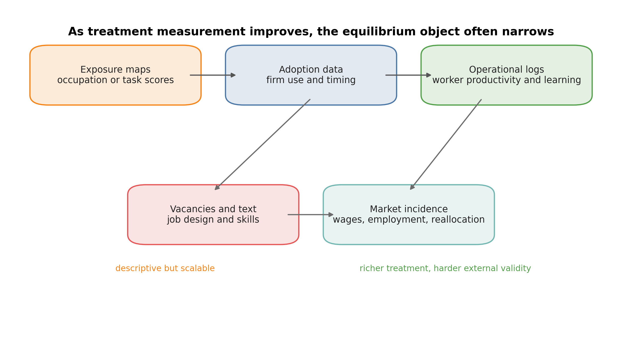
Figure 5:AI measurement sits on a ladder from descriptive exposure to realized adoption to operational productivity logs and finally to market-level incidence. Moving down that ladder usually improves treatment measurement but narrows the equilibrium object that is directly observed.
The cleanest measurement distinction is between public occupation exposure measures and actual use. Public exposure measures scale well and are easy to merge with labor data, but they remain descriptive mappings from task content to predicted technological relevance Felten et al., 2018. Firm adoption data measure realized treatment more directly, but selection into adoption becomes central Aghion et al., 2025. Vacancy data reveal changing labor demand and job design, but postings are not employment Acemoglu et al., 2020. Worker-level field or operational data identify heterogeneity in productivity or learning, but they are often narrow in setting and weak on general equilibrium Brynjolfsson et al., 2025.
Global and comparative evidence
Week 11 should be explicitly comparative. Michaels, Natraj, and Van Reenen show ICT-related skill-demand shifts across eleven countries Michaels et al., 2014. Graetz and Michaels show robot-associated productivity and labor-market patterns across seventeen countries Graetz & Michaels, 2018. Dauth et al. study German labor-market adjustment to robots with strong worker and regional detail Dauth et al., 2021. Aghion et al. add contemporary French firm evidence on how different uses of AI shape labor demand Aghion et al., 2025.
The reason to keep these settings together is not to produce a country catalog. It is to show that institutions, training systems, bargaining structures, sector mix, and mobility shape equilibrium adjustment. Cross-country evidence therefore helps with external validity, but it also warns against taking one design as universal.
Research frontier and extension block
The optional ninety-minute extension block should be longer than usual because this is one of the major shock-and-adjustment weeks in Labor II. A useful frontier map includes at least six open questions.
How much of measured AI exposure predicts realized adoption, and how much remains a descriptive forecast?
When does AI complement weaker or less experienced workers, and when does it mainly increase scale for already-strong workers?
How much technology adjustment runs through wage-setting and rent sharing rather than headcount alone?
Which organizational complements determine whether AI is labor-saving, labor-using, or primarily redistributive inside firms?
What is genuinely new about contemporary AI relative to earlier ICT and robot waves Liu et al., 2025?
Which policies matter most for worker transition support: training subsidies, diffusion policy, wage insurance, or mobility support?
The discipline for frontier work is the same as for canonical papers. Name the identifying variation, the unit of observation, the observed margin, and the equilibrium object that still sits offstage.
Bridge to Week 12
Week 11 studied technology as a shock generated inside production, task choice, and organizational redesign. Week 12 will study trade and offshoring as shocks generated through global goods and production integration. Both weeks are about labor-market adjustment, but the mapping from exposure to incidence differs. Technology shocks often begin with task assignment and adoption inside firms; trade shocks often begin with product-market integration and import or export exposure across firms, industries, and places.
Research Lab
The Week 11 lab follows the standard Reproduce -> Diagnose -> Transfer structure and keeps the bounded student path fully local. The primary anchor is Aghion et al., 2025, where the core teaching object is realized AI adoption by use type inside firms. The challenge anchor is Acemoglu & Restrepo, 2020, where the contrast is a local-labor-market exposure design rather than a within-firm adoption design. The optional extension anchor is Brynjolfsson et al., 2025, which helps students connect worker-level productivity and learning evidence to the broader demand-side and equilibrium framework.
The local handout lives at lab.md. The point of the lab is not to turn students loose on a vague “AI and jobs” exercise. It is to force them to state whether the object is supply-side, demand-side, or market-level; whether the technology measure is exposure or adoption; what the unit of observation is; which labor margin is observed; and which equilibrium margin remains offstage.
Methods Box
Keep these distinctions explicit throughout the week.
Tasks versus occupations: tasks are the economically primitive object in the theory, while occupations are observed bundles that mix many tasks Acemoglu & Autor, 2011.
Exposure versus adoption: exposure measures predicted susceptibility; adoption measures realized use, usually with more selection concerns Felten et al., 2018Aghion et al., 2025.
Within-firm versus market-level evidence: firm evidence is strongest on direct labor-demand responses, while local-market designs are stronger on equilibrium incidence across places Aghion et al., 2025Acemoglu & Restrepo, 2020.
Direct displacement versus indirect productivity and output effects: a negative coefficient on an exposed task margin is not the whole labor-demand effect Acemoglu & Restrepo, 2019.
Historical ICT and robot evidence versus very recent AI evidence: the underlying technologies, diffusion speeds, and observable margins differ Michaels et al., 2014Brynjolfsson et al., 2025.
Skill obsolescence versus skill acquisition: technology can raise the return to learning while making prior task-specific knowledge depreciate faster Bartel & Sicherman, 1998Deming & Noray, 2020.
Public occupation exposure maps versus actual use: descriptive exposure should not be narrated as realized treatment Felten et al., 2018.
Descriptive exposure correlations versus causal adoption evidence: each tells a different part of the labor-market story and neither replaces the other Acemoglu et al., 2020Aghion et al., 2025.
Reading Ladder And References
Ladder A. Core framework
Ladder B. Historical and global evidence
Ladder C. Worker adaptation and labor supply
Ladder D. Contemporary AI, measurement, and frontier directions
Optional frontier extension: Liu et al., 2025
Exercises And Discussion Prompts
Pick one paper from the week and name the identifying variation, unit of observation, observed margin, and key equilibrium margin left offstage.
Suppose a new AI system raises output per worker in a call-center setting. List at least four labor-market objects that could still move in opposite directions: employment, wage inequality, vacancy content, and worker progression are good starting candidates.
Compare Acemoglu & Restrepo, 2020 with Aghion et al., 2025. Which one is closer to exposure, which one is closer to adoption, and which one is closer to market-level equilibrium incidence?
Design a bounded empirical exercise that distinguishes skill obsolescence from skill acquisition using either public occupation cells or a synthetic worker panel.
Reproducibility And Code Lab Note
The bounded pedagogical path lives in lab.md. It is intentionally local and synthetic. Students reproduce a firm-level AI-use design, diagnose the difference between adoption and exposure, and then transfer one exposure idea to a small market-level setting. The smoke test runs only that bounded path.
Slide Companion Note
The canonical Week 11 slide source is 11
Bridge Forward
Use this closing bridge to carry the module’s labor object, mechanism, and evidence into the next course step or research-design exercise.
- Autor, D. H. (2015). Why Are There Still So Many Jobs? The History and Future of Workplace Automation. Journal of Economic Perspectives, 29(3), 3–30. 10.1257/jep.29.3.3
- Autor, D. H. (2022). The Labor Market Impacts of Technological Change: From Unbridled Enthusiasm to Qualified Optimism to Vast Uncertainty. NBER Working Paper 30074. 10.3386/w30074
- Acemoglu, D., & Restrepo, P. (2019). Automation and New Tasks: How Technology Displaces and Reinstates Labor. Journal of Economic Perspectives, 33(2), 3–30. 10.1257/jep.33.2.3
- Acemoglu, D., & Autor, D. (2011). Skills, Tasks and Technologies: Implications for Employment and Earnings. In D. Card & O. Ashenfelter (Eds.), Handbook of Labor Economics (Vol. 4B, pp. 1043–1171). Elsevier. 10.1016/S0169-7218(11)02410-5
- Bartel, A. P., & Sicherman, N. (1998). Technological Change and the Skill Acquisition of Young Workers. Journal of Labor Economics, 16(4), 718–755. 10.1086/209904
- Deming, D. J., & Noray, K. L. (2020). Earnings Dynamics, Changing Job Skills, and STEM Careers. Quarterly Journal of Economics, 135(4), 1965–2005. 10.1093/qje/qjaa021
- Michaels, G., Natraj, A., & Van Reenen, J. (2014). Has ICT Polarized Skill Demand? Evidence from Eleven Countries over Twenty-Five Years. Review of Economics and Statistics, 96(1), 60–77. 10.1162/REST_a_00366
- Acemoglu, D., & Restrepo, P. (2020). Robots and Jobs: Evidence from US Labor Markets. Journal of Political Economy, 128(6), 2188–2244. 10.1086/705716
- Dauth, W., Findeisen, S., Suedekum, J., & Woessner, N. (2021). The Adjustment of Labor Markets to Robots. Journal of the European Economic Association, 19(6), 3104–3153. 10.1093/jeea/jvab012
- Aghion, P., Bunel, S., Jaravel, X., Mikaelsen, T., Roulet, A., & Søgaard, J. (2025). How Different Uses of AI Shape Labor Demand: Evidence from France. AEA Papers and Proceedings, 115, 62–67. 10.1257/pandp.20251047
- Acemoglu, D., Autor, D., Hazell, J., & Restrepo, P. (2020). AI and Jobs: Evidence from Online Vacancies. NBER Working Paper 28257. 10.3386/w28257
- Graetz, G., & Michaels, G. (2018). Robots at Work. Review of Economics and Statistics, 100(5), 753–768. 10.1162/rest_a_00754
- Brynjolfsson, E., Li, D., & Raymond, L. R. (2025). Generative AI at Work. Quarterly Journal of Economics, 140(2), 889–947. 10.1093/qje/qjae044
- Felten, E. W., Raj, M., & Seamans, R. (2018). A Method to Link Advances in Artificial Intelligence to Occupational Abilities. AEA Papers and Proceedings, 108, 54–57. 10.1257/pandp.20181021
- Labaschin, B., Eloundou, T., Manning, S., Mishkin, P., & Rock, D. (2025). Extending “GPTs Are GPTs” to Firms. AEA Papers and Proceedings, 115, 51–55. 10.1257/pandp.20251045