Dynamic Labor Demand and Adjustment Costs
Learning Objectives
By the end of Week 2, students should be able to:
explain why actual employment can remain away from the Week 1 static target when labor adjustment is costly;
distinguish target employment from actual employment, and reduced-form speed-of-adjustment estimates from structural adjustment-cost parameters;
write a dynamic labor-demand problem with adjustment costs and interpret the key state variables;
contrast convex adjustment costs with fixed or nonconvex costs, including the difference between smooth partial adjustment and lumpy inaction;
explain why hours, headcount, hiring, separations, and vacancies need not move at the same horizon;
interpret policy event studies and structural dynamic evidence without confusing timing responses with long-run effects;
connect Week 2 forward to Week 3 on personnel choices inside the firm.
Opening Orientation
The economic question for Week 2 is a direct continuation of Week 1: once the firm has a desired labor target, why does observed employment usually move toward that target gradually rather than instantly?
Bridge
Week 1 derived the firm’s static target. If wages, output demand, technology, or payroll taxes change, the firm has a new desired employment level. Week 2 asks why that destination does not instantly become the observed employment path. Hiring takes screening and onboarding. Firing can trigger legal, organizational, or morale costs. Reassigning workers, changing shifts, or expanding vacancies can be easier than changing core headcount right away Nickell, 1986Hamermesh, 1989.
That makes the basic Week 2 distinction unavoidable: the static benchmark tells us where the firm would like to be, but dynamic labor demand studies how the firm moves from its inherited workforce to that new target. The observed path reflects state dependence, the availability of alternative margins, and the firm’s expectations about whether the shock will persist.
This week remains firmly inside the firm. It does not yet build a full search equilibrium, bargaining model, or monopsony framework. Those arrive later. The point here is narrower and foundational: before labor markets can be matched or bargained over, firms still face a dynamic employment problem. Week 3 will take that dynamic firm and ask how incentives, internal labor markets, and promotion structures reshape its personnel choices.
Field Core
From target employment to actual employment
Week 1 gave the static benchmark. We can summarize it as a target-employment object:
Equation (1) is the correct bridge back to Week 1. The target depends on wages, productivity, output demand, and other state variables. Week 2 begins because actual employment need not equal each period. Firms inherit yesterday’s workforce, not a blank slate.
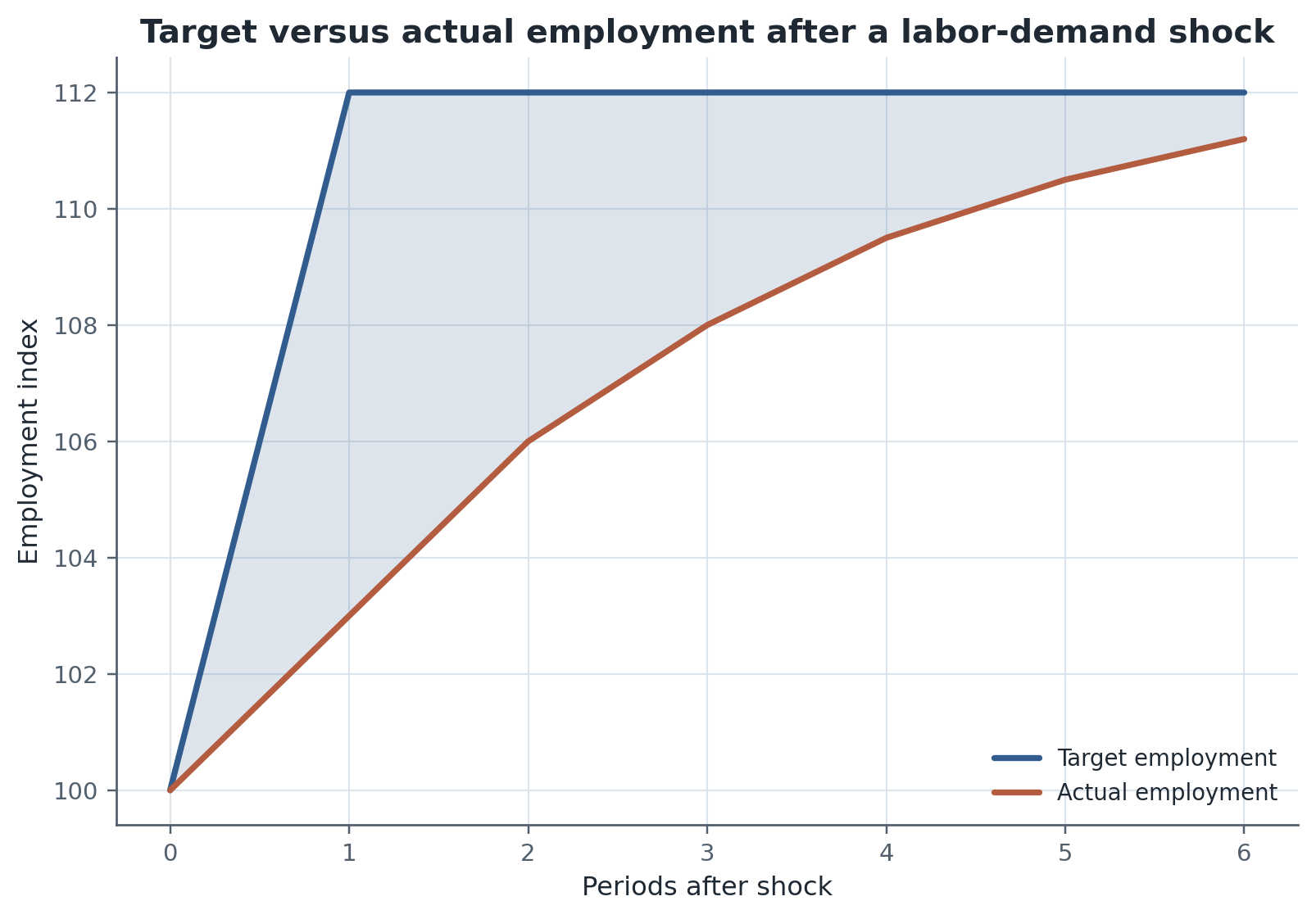
Figure 1:Target versus actual employment after a positive labor-demand shock. The gap between the two is the central Week 2 object: the firm knows where it wants to go, but it gets there gradually.
Figure Figure 1 makes the main conceptual move visible. The empirical object is not just the new target after a shock. It is the gap between actual and target employment, how quickly that gap closes, and which margins close it first.
This is also the right place to introduce horizon language. In the short run, firms often move hours, overtime, or temporary labor before they move permanent headcount. In the medium run, hiring and separations begin to reshape the workforce. In the long run, capital, task allocation, and organizational structure may also adjust. A single employment estimate without a horizon is therefore incomplete Shapiro, 1986Hamermesh, 1989.
The dynamic firm problem
The standard dynamic benchmark writes the firm’s problem as
where collects wages, demand, productivity, policy, and other states. Equation (2) says that labor demand is dynamic because employment today changes both current profits and tomorrow’s feasible choices. The inherited workforce is a state variable, not just yesterday’s accounting outcome.
Three ideas follow immediately.
Employment persistence is not automatically proof of adjustment costs. Persistence can also reflect persistent shocks, measurement timing, or other omitted states.
The cost function is the central Week 2 object because it determines how painful it is to move employment.
If hours, overtime, vacancies, or temporary workers are cheaper to vary than core headcount, those margins will absorb more of the short-run response.
Table 1:Adjustment-cost taxonomy for dynamic labor demand
| Cost structure / friction | Core intuition | Typical dynamic signature | Main labor margin implications | What researchers try to identify |
|---|---|---|---|---|
| Convex adjustment costs | Small changes are cheap; large changes are increasingly costly | Smooth partial adjustment toward target employment | Frequent modest changes in hours or headcount | Speed of adjustment, short-run vs long-run elasticity |
| Fixed / nonconvex adjustment costs | Any change triggers a fixed reorganization or hiring/firing cost | Inaction punctuated by lumpy jumps | Spikes in hiring/firing, long spells of no change | Inaction bands, hazard of adjustment, lumpiness |
| Quasi-fixed labor | Some workers or employment relationships are costly to vary quickly | Persistence even when output fluctuates | Firms use hours, overtime, temps, or inventories first | Whether headcount is the true flexible margin |
| Hiring costs | Recruiting, screening, onboarding, and training are costly | Sluggish expansion after positive shocks | Vacancies rise before employment rises | Hiring frictions versus true demand weakness |
| Firing / separation costs | Layoffs are legally, financially, or organizationally costly | Slow contraction after negative shocks | Downward rigidity in headcount, more hours compression | Asymmetry between expansion and contraction |
| Uncertainty / option value of waiting | Firms delay irreversible changes when the environment is noisy | Short-run hesitation and delayed response | Vacancies or hours adjust before permanent staff | Distinguishing delay from low desired employment |
Table Table 1 summarizes the main friction types. The key distinction is not merely between “fast” and “slow” firms. It is between cost structures that imply smooth adjustment and cost structures that imply inaction punctuated by jumps.
Convex adjustment costs and partial adjustment
The cleanest benchmark uses convex costs, often quadratic in employment changes. In that case, large employment changes are disproportionately expensive, so the firm spreads adjustment across time Nickell, 1986Shapiro, 1986.
Equation (3) is the textbook partial-adjustment law. If , the firm jumps immediately to target. If is small, adjustment is gradual. Empirically, is often estimated as a reduced-form speed-of-adjustment parameter. It is useful, but it is not itself a primitive structural cost parameter. Mapping from to deep costs requires stronger model discipline than a one-equation estimate provides Hamermesh, 1989.
Convex costs imply frequent but modest changes. That matters for policy interpretation. When a payroll-tax cut lowers labor cost today, the employment response may unfold over multiple horizons even if the new target is known immediately. Short-run incidence can therefore differ sharply from medium-run and long-run incidence.
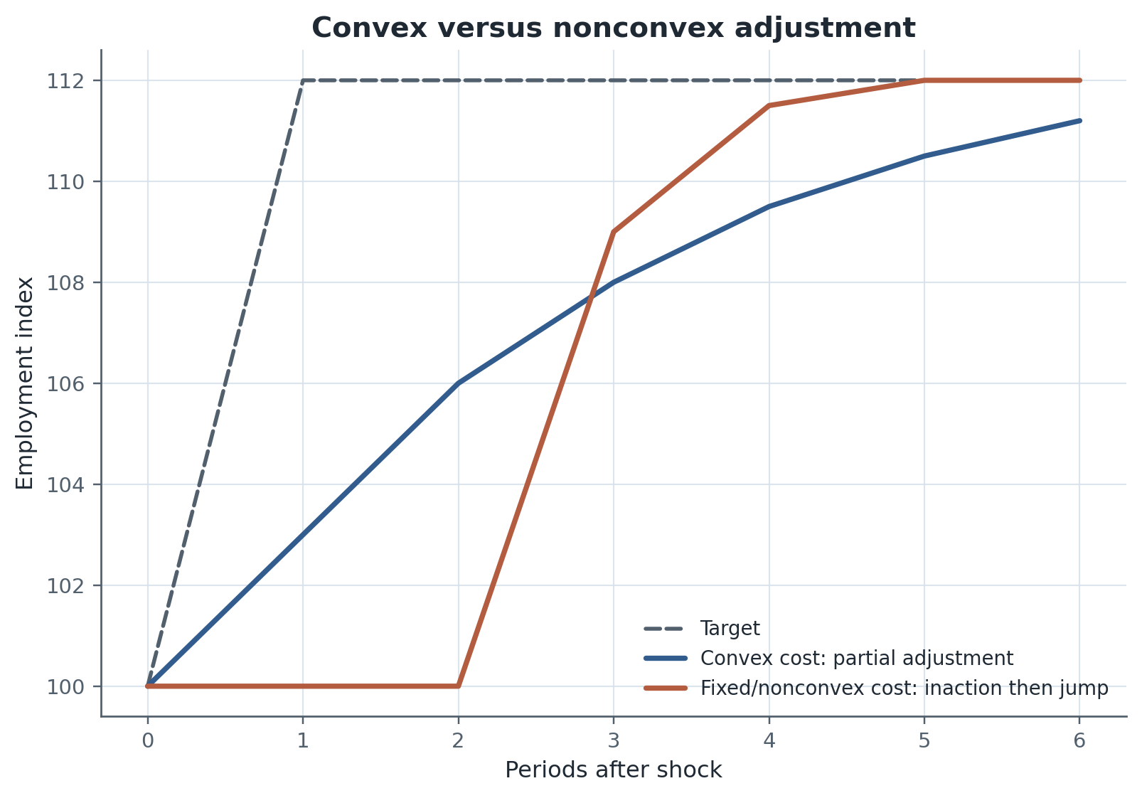
Figure 2:Convex costs generate smooth partial adjustment, while fixed or nonconvex costs generate inaction followed by larger jumps.
Figure Figure 2 highlights what convex costs do not predict. If the data show many zero adjustments combined with occasional large spikes, the convex benchmark is incomplete.
Fixed and nonconvex costs, inaction, and lumpiness
When adjustment triggers a fixed reorganization cost, a hiring cost, or a firing cost that does not scale smoothly with the size of the change, firms may wait until the gap is large enough to justify moving. A compact threshold representation is
Equation (4) is not a full model, but it captures the central intuition behind nonconvex adjustment. Small shocks generate inaction. Large shocks generate lumpy adjustments. This is the language students need before reading plant-level evidence on hazards, zeros, and spikes in employment change Caballero et al., 1997.
The substantive contrast with convex costs is sharp.
Convex costs predict smooth employment paths and many small adjustments.
Fixed or nonconvex costs predict long spells of no change and occasional large adjustments.
Firing costs can generate asymmetry: contraction after negative shocks may be slower or differently timed than expansion after positive shocks Bentolila & Bertola, 1990.
Micro lumpiness does not imply aggregate chaos. Many plants can adjust at different times, so aggregate employment still looks smoother than establishment-level behavior. That is one reason macro employment persistence alone is not enough to identify the micro cost structure.
Which margin adjusts first?
Dynamic labor demand is not only about how much employment moves. It is also about which margin moves first. Hours and overtime are often quicker to vary than permanent headcount. Hiring and vacancies are more informative after positive shocks; layoffs and separations are more informative after negative shocks. Temporary labor can buffer the core workforce. Labor hoarding means a firm may keep headcount high after a temporary downturn while reducing hours, effort, or utilization.
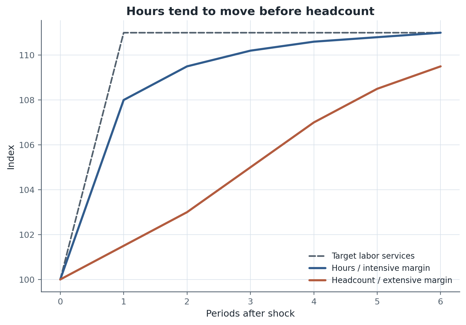
Figure 3:Hours often absorb more of the short-run response than headcount. That is why headcount-based estimates alone can understate early labor-demand adjustment.
Figure Figure 3 is a warning against one-margin empirics. A weak contemporaneous employment effect does not imply that labor demand failed to respond. It may imply that the firm used the intensive margin first.
Table 2:Observed labor margins and what they reveal
| Observed margin | What it can reveal | What it can miss | Why it matters for interpretation |
|---|---|---|---|
| Headcount / employment | Permanent staffing adjustment | Intensive-margin responses and hidden labor hoarding | A weak headcount response does not imply no labor-demand response |
| Hours worked | Short-run flexibility and utilization of existing workers | Longer-run workforce reorganization | Hours often move before employment |
| Hires / vacancies | Expansion frictions and recruiting constraints | Contraction-side rigidity | Useful for separating positive-shock adjustment from weak demand |
| Separations / layoffs | Contraction margins and firing costs | Expansion frictions | Especially informative for asymmetry and employment protection |
| Overtime / temporary labor | Buffer-stock use of flexible labor inputs | Permanent headcount strategy | Helps explain why firms delay changes in core employment |
| Wages / compensation | Possible rent sharing or internal adjustment | True quantity adjustment if wages are sticky | Dynamic incidence can be split between wages and employment |
| Capital or production | Complementary firm response outside labor | Pure labor-market mechanism | Ignoring other margins can bias labor-demand interpretation |
Table Table 2 should be read before any empirical result is interpreted. The first question is always: what labor margin is observed? The second is: which margins were available but unobserved?
Empirical designs and what they identify
Week 2 evidence is easiest to organize by identifying variation rather than by chronology.
Table 3:Empirical design map for Week 2
| Design family | Source of variation | Main observed margin | Dynamic object identified | Main limitation |
|---|---|---|---|---|
| Plant or establishment panels | Repeated firm-level outcomes over time | Employment, hours, hires, separations | Persistence, hazards, lumpiness, partial adjustment | Hard to separate true frictions from unobserved shocks |
| Payroll-tax or labor-cost reforms | Policy-induced changes in labor cost | Employment, wages, hours, profits over event time | Short-run and longer-run incidence paths | Firms may simultaneously adjust prices, capital, or workforce composition |
| Uncertainty shocks / expectation surveys | Changes in perceived uncertainty or hypothetical shocks | Expected employment, investment, production | Delay, option value of waiting, heterogeneity in costs | Expectations may not equal realized behavior |
| Structural dynamic estimation | Model-based mapping from states to choices | Firm adjustment paths | Deep cost parameters and counterfactuals | Identification depends on model discipline and state measurement |
| Event-study timing designs | Pre/post policy or shock path | Employment path by horizon | Response dynamics at different horizons | Parallel-trends assumptions may fail at long horizons |
Plant and establishment panels track repeated outcomes for the same firm or production unit. The identifying variation comes from within-unit changes over time, and the observed margins are often employment, hours, hires, or separations. These designs are useful for persistence, hazard, and lumpiness, but unobserved shocks can still masquerade as adjustment frictions Hamermesh, 1989Caballero et al., 1997.
Policy timing designs use labor-cost reforms or payroll-tax changes as the shock. The identifying variation is a change in labor cost, and the observed margin may include employment, hours, wages, or profits over event time. These designs identify dynamic incidence paths rather than a timeless elasticity Saez et al., 2019.
Survey or expectation-based designs are especially useful when the question is whether uncertainty changes the timing of adjustment. In Dibiasi et al., 2025, the identifying variation comes from differences in uncertainty and firm beliefs, while the observed objects are expected and realized employment responses. That is informative about delay and state dependence, but it is not the same as observing every margin of actual headcount change in administrative payroll records.
Structural dynamic estimation goes one step further by imposing a model like Equation (2) and estimating deep cost parameters. That can support counterfactual policy analysis, but only if the state space, the choice set, and measurement of margins are credible. This is why a reduced-form speed-of-adjustment estimate and a structural cost estimate answer related but distinct questions.
Policy timing and incidence over the adjustment path
Dynamic labor demand matters for policy because incidence is a path, not just an endpoint. If a payroll tax changes at , the relevant object is
Equation (5) forces the timing question into the notation. The contemporaneous effect can be modest if firms first adjust hours, vacancies, or prices. Medium-run effects may be larger as headcount changes accumulate. Long-run effects may differ again once capital and organization adjust.
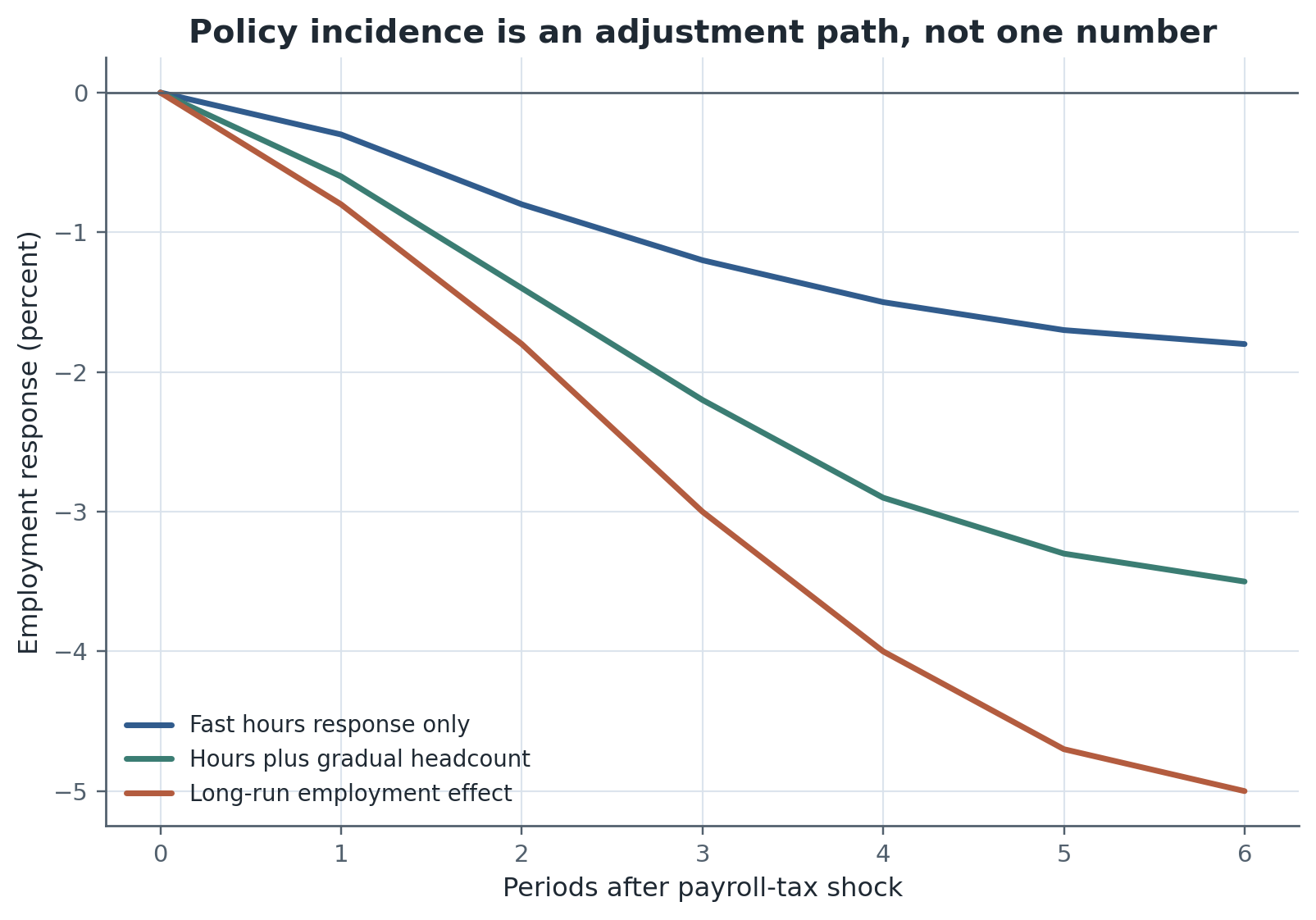
Figure 4:The employment effect of a labor-cost shock often builds over time. Short-run, medium-run, and long-run incidence need not coincide.
Figure Figure 4 is the clean bridge from theory to applied policy work. Saez et al., 2019 is useful here because the identifying variation is a payroll-tax reform, the observed margins include both wages and employment, and the key result is dynamic incidence rather than a single static elasticity. The same reform can look small in the short run and substantial over longer horizons because the firm’s adjustment margins are sequenced.
The dynamic policy lesson is broader than payroll taxes. Employment protection, firing costs, and hiring subsidies all reshape the timing margin. The central Week 2 habit is therefore to report both the shock and the horizon.
Research Lab
The frontier lesson from Week 2 is that observed persistence is economically ambiguous until we name the target, the horizon, and the observed margin. A plant panel with many zero employment changes points toward nonconvex adjustment, but it may also reflect uncertainty, measurement intervals, or the availability of off-margin responses. A policy event study with a flat contemporaneous estimate may still hide meaningful medium-run employment adjustment if firms move hours or wages first.
Dibiasi et al., 2025 is a strong lab anchor because it pushes students to interpret dynamic responses through firm beliefs and uncertainty rather than through one-shot elasticities alone. Caballero et al., 1997 is the complementary challenge anchor because it asks what aggregate employment dynamics imply once micro-level inaction and lumpiness are present.
Optional extension block
One optional extension is uncertainty and the option value of waiting. If adjustment is partly irreversible, firms may delay employment changes when the environment is noisy even if the static target has already shifted. This is the cleanest route from dynamic labor demand into beliefs, expectations, and survey evidence Dibiasi et al., 2025.
The second optional extension is structural estimation. Here the goal is to recover deep adjustment-cost parameters rather than only a reduced-form response speed. That move is valuable for counterfactual policy analysis, but it requires stronger assumptions about the state space, the firm’s information set, and which margins are observed.
Methods Box
Week 2 only works if the empirical language stays disciplined.
Target employment is the Week 1 object; actual employment is the Week 2 object.
Convex costs imply partial adjustment; fixed or nonconvex costs imply inaction bands and lumps.
Hours versus headcount and hiring versus firing are not interchangeable margins.
Short-run, medium-run, and long-run responses can differ even under the same eventual target.
A reduced-form speed-of-adjustment estimate is not the same object as a structural cost parameter.
Policy event studies identify dynamic timing responses to a shock; structural dynamic models try to recover primitives that support counterfactuals.
Do not report an empirical result without naming both the identifying variation and the observed margin.
Reading Ladder And References
Bucket A. Dynamic benchmark
Nickell, 1986 for the canonical field-style overview of dynamic labor-demand models.
Shapiro, 1986 for a dynamic factor-demand benchmark that helps students see why adjustment speed is an equilibrium object inside the firm.
Hamermesh, 1989 for the structure of adjustment costs and the distinction between reduced-form adjustment patterns and underlying cost primitives.
Bucket B. Adjustment frictions and firing costs
Bentolila & Bertola, 1990 for the logic of firing costs and asymmetric adjustment.
Caballero et al., 1997 for the connection between establishment-level lumpiness and aggregate employment dynamics.
Bucket C. Modern measurement of dynamic frictions
Dibiasi et al., 2025 for evidence linking uncertainty, firm beliefs, and adjustment costs to employment timing.
Bucket D. Policy timing and incidence bridge
Saez et al., 2019 for payroll-tax incidence over the adjustment path and the bridge from dynamic labor demand to later wage-setting weeks.
Exercises And Discussion Prompts
Use Equations (1) and (3) to explain why a contemporaneous employment estimate can understate the eventual effect of a labor-cost shock.
What features of plant-level data would make you favor Equation (4) over Equation (3)?
Why can two studies of the same reform disagree if one observes hours and the other observes headcount?
In Table Table 3, which designs speak most directly to policy timing, and which speak most directly to structural cost parameters?
How does Week 2 change the interpretation of the Week 1 target employment object?
Reproducibility And Code Lab Note
The Week 2 lab follows the standard Reproduce -> Diagnose -> Transfer structure. The bounded reproduction path uses a local synthetic firm panel inspired by Dibiasi et al., 2025 so students can trace target versus actual employment, hours, and uncertainty without confidential microdata. The diagnose step asks them to name the identifying variation, the observed margin, and the implied dynamic object. The transfer step then compares convex and nonconvex adjustment paths with Caballero et al., 1997 as the challenge anchor and Saez et al., 2019 as the optional policy-timing extension. The local handout lives at lab.md.
Slide Companion Note
The slide deck at 02
Bridge Forward
Use this closing bridge to carry the module’s labor object, mechanism, and evidence into the next course step or research-design exercise.
- Nickell, S. J. (1986). Dynamic Models of Labour Demand. In O. C. Ashenfelter & R. Layard (Eds.), Handbook of Labor Economics (Vol. 1, pp. 473–522). Elsevier.
- Hamermesh, D. S. (1989). Labor Demand and the Structure of Adjustment Costs. The American Economic Review, 79(4), 674–689.
- Shapiro, M. D. (1986). The Dynamic Demand for Capital and Labor. The Quarterly Journal of Economics, 101(3), 513–542.
- Caballero, R. J., Engel, E. M. R. A., & Haltiwanger, J. C. (1997). Aggregate Employment Dynamics: Building from Microeconomic Evidence. The American Economic Review, 87(1), 115–137.
- Bentolila, S., & Bertola, G. (1990). Firing Costs and Labour Demand: How Bad Is Eurosclerosis? The Review of Economic Studies, 57(3), 381–402.
- Saez, E., Schoefer, B., & Seim, D. (2019). Payroll Taxes, Firm Behavior, and Rent Sharing: Evidence from a Young Workers’ Tax Cut in Sweden. American Economic Review, 109(5), 1717–1763. 10.1257/aer.20171937
- Dibiasi, A., Mikosch, H., & Sarferaz, S. (2025). Uncertainty Shocks, Adjustment Costs, and Firm Beliefs: Evidence from a Representative Survey. American Economic Journal: Macroeconomics, 17(3), 36–73. 10.1257/mac.20220318