Search, Matching, Turnover, and Unemployment
Learning Objectives
By the end of Week 4, students should be able to:
explain why search frictions generate unemployment, vacancies, turnover, and dispersion in worker outcomes;
distinguish worker flows from job flows, and distinguish separations, layoffs, job destruction, and churning;
derive a compact matching-function and flow-balance framework and interpret worker-side versus vacancy-side hazards;
explain why separations, job-finding, vacancy-filling, and job-to-job mobility are distinct empirical objects;
describe how on-the-job search and job ladders change the interpretation of worker mobility and wage growth;
distinguish observed duration dependence from causal unemployment effects and dynamic selection;
evaluate search evidence by naming the identifying variation, the unit of observation, the observed margin, and the most important unobserved object.
Opening Orientation
The economic question for Week 4 is the first major market-interaction question in Labor II: once firms must search for workers and workers must search for jobs, how are hiring, separations, turnover, job-to-job mobility, and unemployment jointly determined?
Bridge
Weeks 1 through 3 stayed mostly inside the firm. Week 1 studied the firm’s static labor-demand problem, Week 2 studied how the firm adjusts employment over time, and Week 3 studied how the firm organizes, promotes, and retains workers internally. Week 4 changes the unit of analysis. The main object is no longer only the firm’s internal labor problem. It is the frictional labor market in which workers search imperfectly, firms post vacancies imperfectly, meetings take time, separations occur, and unemployment is a flow equilibrium outcome rather than a static stock Rogerson et al., 2005Pissarides, 2000.
That move requires a tighter vocabulary than students often bring into the room. Unemployment is a worker-state object. Vacancies are a firm-side recruiting object. Job destruction is a job-flow object. Job-to-job mobility is neither a layoff rate nor a vacancy statistic. Churning is worker reallocation beyond net job creation. If we collapse these together, the whole week becomes conceptually muddy before any equation appears.
The bridge back to Week 3 is also substantive rather than cosmetic. Personnel practices affect quits, retention, internal mobility, and recruiting pressure even if Week 3 mostly analyzed choices inside one firm. Week 4 asks how those firm-side choices aggregate into worker flows across firms and states. Week 5 then takes the next logical step: once outside options, vacancies, and mobility frictions matter, wages can no longer be treated as purely competitive objects.
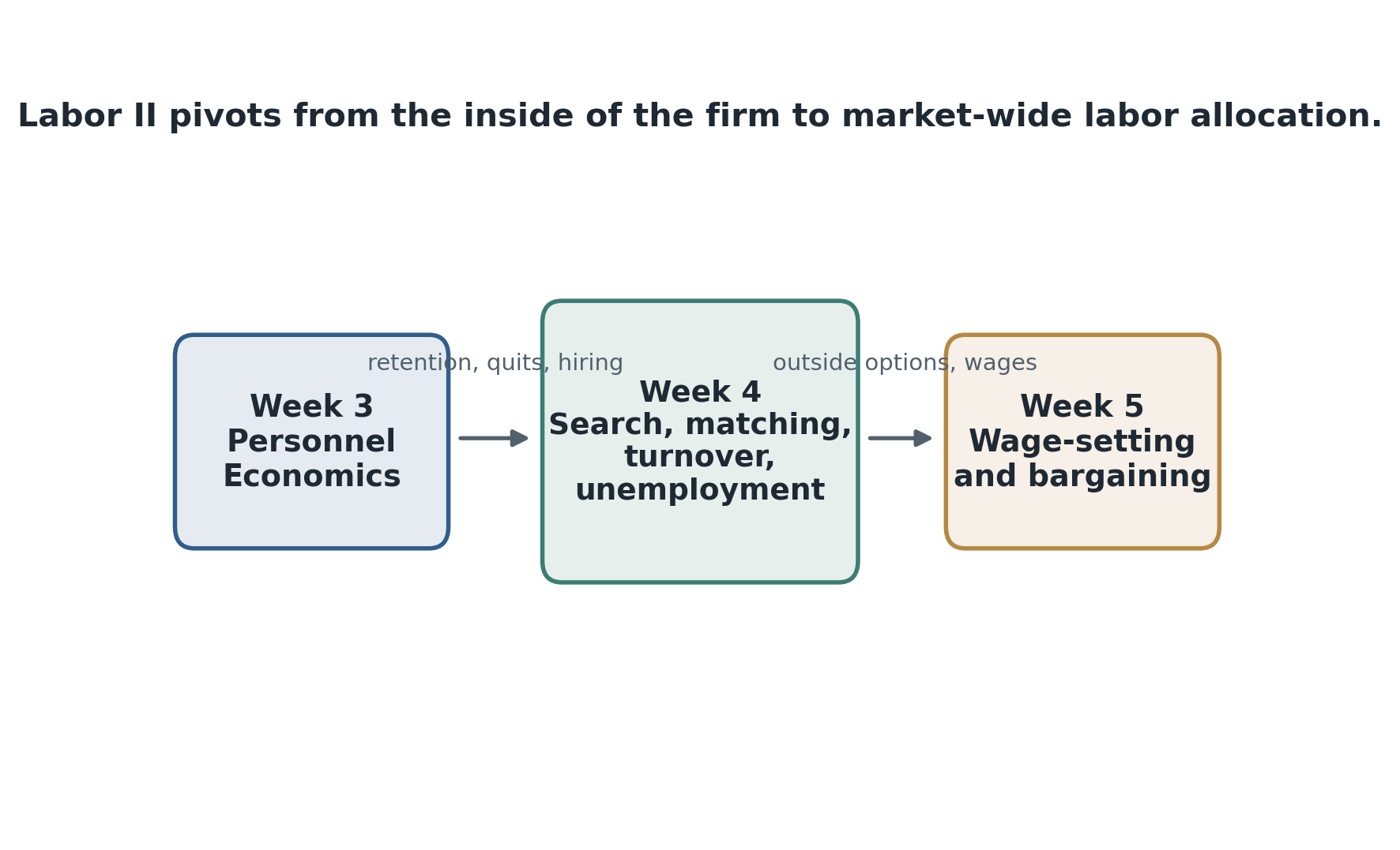
Figure 1:Search and matching is the bridge from the inside of the firm to market-wide labor allocation. Week 4 moves from internal labor markets to worker flows, then forward to wage-setting, bargaining, and labor market power.
Table 1:Search objects map for Week 4
| Object | Definition | Typical data source | Why it matters | Common confusion to avoid |
|---|---|---|---|---|
| Job-finding rate | Hazard from unemployment to employment | CPS flows, admin records | Governs outflow from unemployment | Not the same as vacancy-filling |
| Separation rate | Hazard from employment to unemployment or nonemployment | CPS flows, employer records | Governs inflow into unemployment | Not all separations are layoffs |
| Vacancy-filling rate | Hazard from vacancy to match | JOLTS, firm vacancy data | Captures recruiting congestion | Not directly observable from worker data |
| Job-to-job transition rate | Hazard from one employer to another without unemployment | Matched employer-employee data, CPS supplements | Core object for job ladders and sorting | Not captured by unemployment-only models |
| Churning / excess worker reallocation | Worker flows beyond net employment changes | Employer-level administrative data | Separates internal turnover from net job creation | Not the same as job destruction |
| Unemployment duration gradient | Relationship between spell length and later outcomes or hazards | Survey panels, admin data, search apps | Central to causal vs selection debates | Duration dependence need not be causal |
Figure Figure 1 and Table Table 1 should anchor the opening discussion. The point is not to memorize a taxonomy. The point is to see that different data and different theories speak to different flow objects.
Field Core
Why search frictions matter
The cleanest benchmark is that workers and firms do not meet costlessly. Search takes time, information is incomplete, and acceptance decisions depend on outside options. A matching technology summarizes how workers and vacancies meet:
where is the number of unemployed job seekers and is the number of open vacancies. Equation (1) is deliberately reduced form. It is a meeting technology, not yet a full theory of who searches intensely, which jobs are targeted, or why wages differ Rogerson et al., 2005.
The same meeting technology produces distinct hazards for workers and vacancies:
Equation (2) is the first major Week 4 distinction. is the job-finding rate faced by unemployed workers. is the vacancy-filling rate faced by firms. Both come from the same aggregate matching object, but they answer different questions. The worker asks, “How likely am I to exit unemployment?” The firm asks, “How likely is my vacancy to be filled?” This is why labor-market tightness matters: the same market can be good for workers and hard for recruiters at the same time.
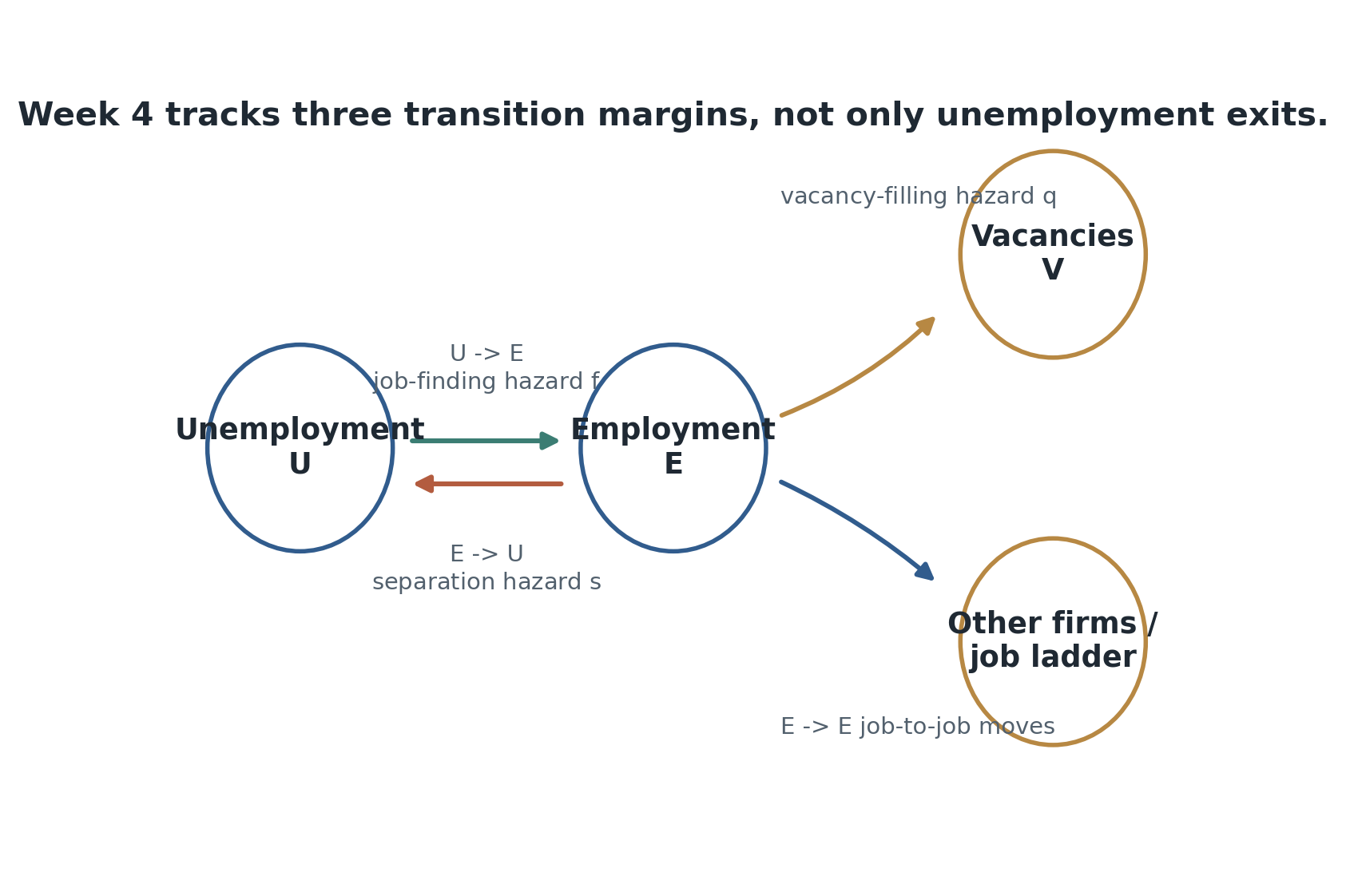
Figure 2:Week 4 requires separate attention to unemployment-to-employment, employment-to-unemployment, and employment-to-employment flows. Worker-side hazards and vacancy-side hazards are different objects even when they are generated by the same meeting environment.
Figure Figure 2 should be read together with Equation (2). Search theory is not only about the U-to-E arrow. The E-to-U and E-to-E arrows are central to turnover, job ladders, and later wage-setting.
Flow unemployment and steady-state accounting
Unemployment is a stock, but it is governed by flows. Let denote the hazard from employment to unemployment. Then unemployment evolves according to
Equation (3) is the accounting backbone of the week. Unemployment rises when inflows from employment exceed outflows to jobs. It falls when job finding dominates separation. In steady state, the corresponding stock relation is
Equation (4) is simple enough to hide an important lesson: unemployment depends jointly on separations and job finding. A labor market can have high unemployment because finding jobs is hard, because jobs end frequently, or because both are true. This is why a theory or policy discussion that treats separation as a nuisance term is incomplete Mortensen & Pissarides, 1994Pissarides, 2000.
The matching function is also not enough by itself to interpret shifts in unemployment and vacancies. Suppose the Beveridge curve appears to shift outward. That can mean lower matching efficiency, but it can also reflect changed composition of job seekers, changed recruiting behavior, or greater mismatch between worker search and vacancy requirements. Hall & Schulhofer-Wohl, 2018 is a central anchor precisely because it pushes students to separate matching efficiency from job-seeker composition.
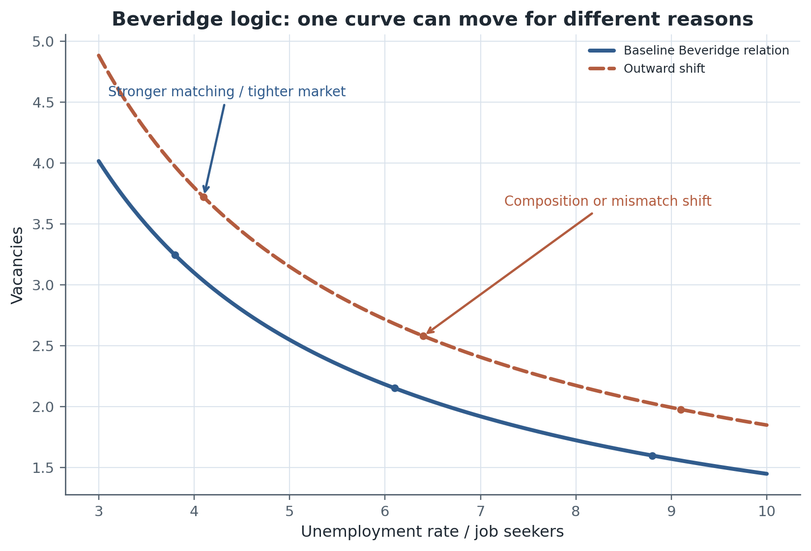
Figure 3:The Beveridge curve organizes unemployment and vacancies, but a shift in the curve is not automatically a pure efficiency shock. Composition of job seekers, recruiting intensity, and mismatch can move the same reduced-form relationship.
Figure Figure 3 belongs here because it disciplines interpretation. Matching efficiency is an unobserved object inferred from observed stocks and flows; it is not directly visible in vacancy and unemployment series alone.
Separations, turnover, job destruction, and churning
Week 4 should spend as much time on inflows into unemployment as on outflows from it. A separation is any worker-level end of an employment spell. A layoff is a particular kind of employer-initiated separation. Job destruction is a job-flow concept: a position disappears. Churning or excess worker reallocation is worker turnover in excess of what net employment change requires. A plant can have stable headcount and still exhibit heavy worker replacement, restructuring, and hiring pressure.
Table 2:Flows, separations, and margins map for Week 4
| Margin | Worker-side interpretation | Firm-side interpretation | Main theory block | Main empirical challenge |
|---|---|---|---|---|
| E → U | Job loss, layoff, quit into unemployment | Separation decision, job destruction, retention failure | Flow unemployment, endogenous destruction | Distinguishing quits, layoffs, and displacement |
| U → E | Reemployment | Vacancy filling from nonemployment pool | Matching, search effort, reservation wages | Composition of searchers and vacancies |
| E → E | Upward or lateral mobility without unemployment | Poaching, outside offers, retention pressure | On-the-job search, job ladders | Need linked worker-firm or panel flow data |
| Stable employment with internal turnover | Replacement hiring, reorganization | Churning, restructuring, personnel adjustment | Turnover and excess reallocation | Net employment masks gross flows |
| Long unemployment spell | Search friction, low hazard, or dynamic selection | Reduced outside-option pressure on firms | Duration dependence, beliefs, scarring | Causal duration effects vs heterogeneity |
| Reemployment wage / job quality | Match quality after nonemployment | Selection into lower- or higher-quality firms | Reservation wages, selective hiring, scarring | Past wage, firm quality, and occupation choice are jointly determined |
Table Table 2 is useful because it keeps worker-side and firm-side language aligned. The E-to-U margin is not the same as job destruction. Quits into other jobs do not pass through unemployment. Replacement hiring can be heavy even when net employment is flat. These are precisely the cases where gross flows contain the real labor-market action.
Mortensen & Pissarides, 1994 remains the canonical theoretical reference because job creation and job destruction are jointly determined in equilibrium, not appended after the fact. But this is also where Labor II should stay labor-focused. What matters for students is that separations respond to plant shocks, product demand, personnel policies, management quality, retention effort, and cyclical conditions. When bad matches dissolve or firms reorganize, unemployment dynamics move even if the aggregate vacancy stock barely changes.
Churning deserves explicit treatment because it separates two ideas students often conflate. Net job creation tells us whether a firm is expanding or contracting. Churning tells us whether the incumbent workforce is being reshuffled beneath a stable employment total. That makes churning a natural bridge back to Week 3 personnel economics: internal organization affects who stays, who exits, and how often the firm must recruit replacements.
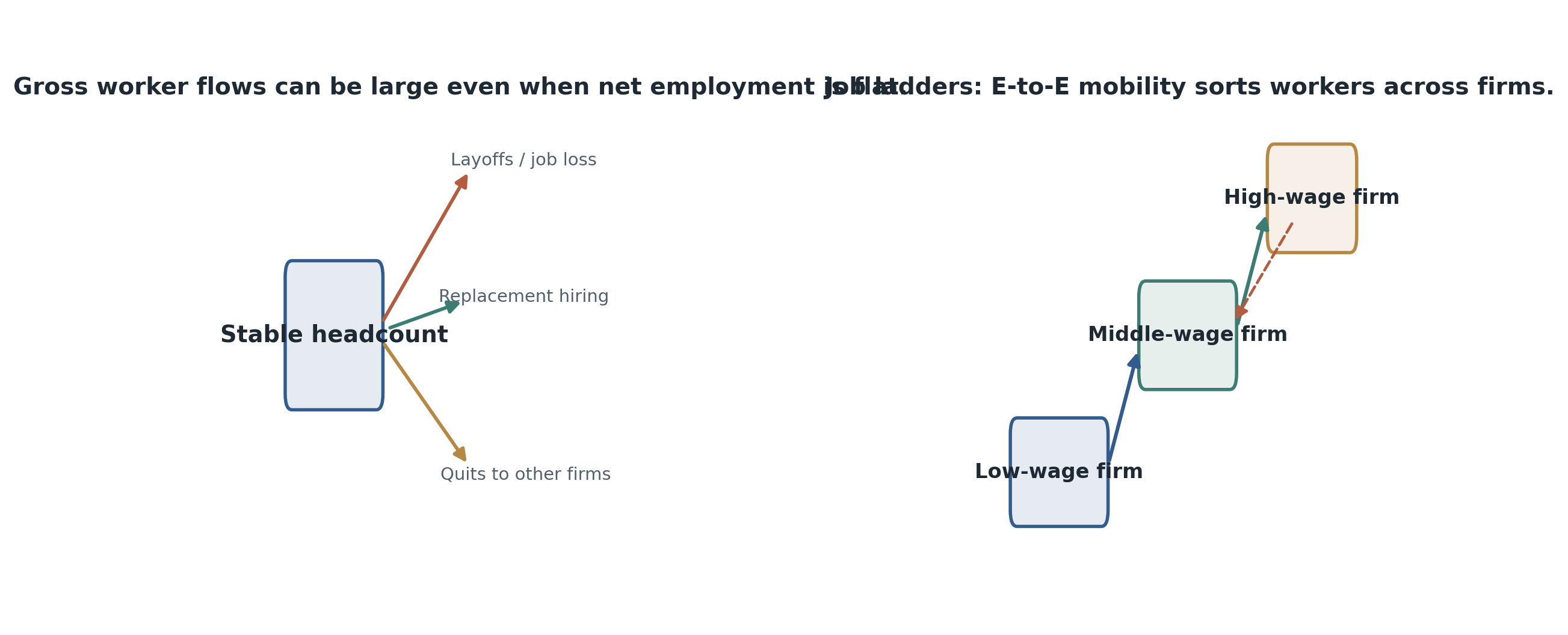
Figure 4:Separations, job destruction, churning, and job ladders are related but not interchangeable. Net employment can stay flat while firms destroy jobs, create new ones, and replace workers through quits, layoffs, and poaching.
Job-to-job transitions, on-the-job search, and job ladders
One of the biggest conceptual upgrades in a serious search week is to stop treating unemployment as the only transition state that matters. Many important labor-market moves occur directly from one employer to another. Those E-to-E transitions are central for wage growth, sorting, firm quality, and later monopsony reasoning.
A compact hazard object for on-the-job search is
where is current compensation, is worker type, is market tightness or business-cycle conditions, and firm quality summarizes nonwage job attributes. Equation (5) keeps the Week 4 mobility discussion disciplined. Employed search depends on both the current job and the outside market.
This is where Burdett & Mortensen, 1998 enters. Once workers can search while employed, better firms poach workers from worse firms, wage growth can occur through outside offers, and job ladders become an equilibrium mobility object rather than a descriptive metaphor. Haltiwanger et al., 2018 is the ideal empirical bridge because the unit is worker transitions across firms, the variation is cyclical and cross-firm, the observed margin is job-to-job upgrading, and the hardest unobserved object is the full opportunity set available to the worker at the time of the move.
The distinction between U-to-E and E-to-E flows also changes how we think about business cycles. When the market weakens, the first visible adjustment may be fewer upward job-to-job moves rather than a dramatic spike in unemployment exits from firms. Job ladders can therefore flatten before unemployment fully rises. That is one reason search theory is not just a theory of unemployment; it is also a theory of mobility and sorting across firms.
Unemployment duration, search intensity, and the consequences of unemployment
Observed unemployment duration is not a sufficient statistic for worker damage. Long spells may reflect declining search effort, employer screening against long durations, worsening beliefs, liquidity pressure, reservation-wage adjustment, or dynamic selection of harder-to-place workers into the remaining unemployment pool.
A compact reduced-form outcome object is
where is unemployment duration and can denote wages, firm quality, or occupation quality after reemployment. Equation (6) is useful because it highlights the main Week 4 warning: an observed duration gradient is not automatically a causal unemployment effect.
Kroft et al., 2013 is an important design anchor because it uses randomized variation in callback environments to study duration dependence in employer responses. Faberman & Kudlyak, 2019 and Mueller et al., 2021 are equally important because they keep search intensity and beliefs in view rather than treating the unemployed as mechanically identical job seekers. The unit in these papers is not a vacancy stock; it is a worker, application, or spell. The observed margins are applications, search effort, expectations, or callbacks. The key unobserved object is often the worker’s full feasible set of jobs and search technologies.
The consequences of unemployment also extend beyond the exit hazard. Schmieder et al., 2016 and Nekoei & Weber, 2017 make clear that longer nonemployment can change later wages and job quality, while Huckfeldt, 2022 shows why recession timing matters for scarring and recovery. The central lesson for Week 4 is modest but important: unemployment is not a neutral waiting room. It can alter later match quality, occupation, earnings trajectory, and even the distribution of firms willing to hire the worker.
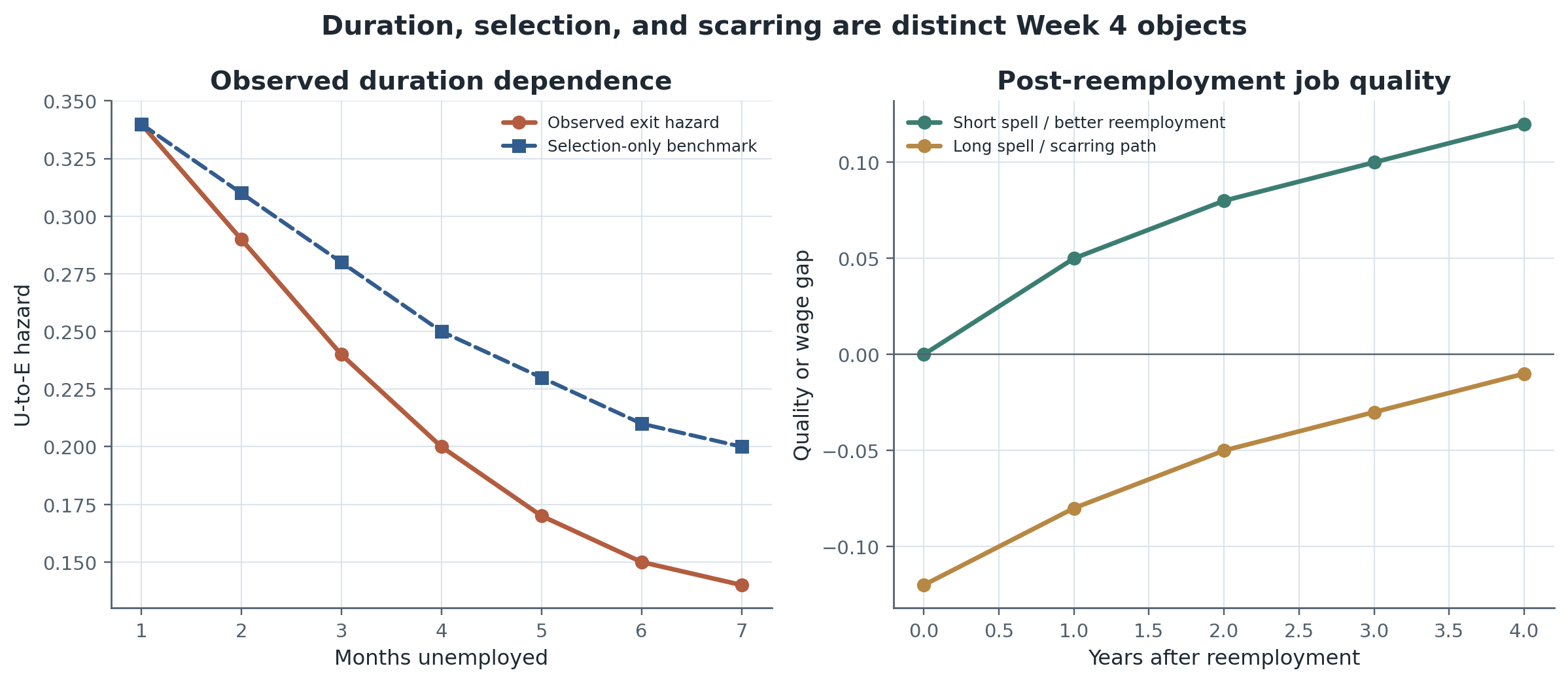
Figure 5:Observed duration dependence can arise from causal unemployment effects, changing search behavior, employer screening, and dynamic selection. The consequences of unemployment therefore include both exit hazards and post-reemployment job quality.
Data and empirical designs: how search empirics identify frictions
Week 4 evidence is easier to teach when organized by design rather than by chronology.
Table 3:Identification and evidence map for Week 4
| Empirical design | Variation used | Margin identified | Best use in this lecture | Main limitation |
|---|---|---|---|---|
| CPS-style transition accounting | Month-to-month labor-force status flows | U-E, E-U, sometimes E-E approximations | Flow decomposition and unemployment accounting | Coarse statuses and recall/misclassification issues |
| Vacancy series / Beveridge evidence | Vacancies over time or across places | Vacancy-filling and matching efficiency patterns | Matching efficiency and congestion | Composition of job seekers usually unobserved |
| Matched employer-employee administrative data | Worker moves across firms/jobs | Job ladders, sorting, churning, separations | On-the-job search and firm-quality mobility | Access and portability are hard |
| Online search/application data | Within-spell application behavior | Search intensity and hazard responses | Search effort, duration, and vacancy targeting | Coverage and representativeness |
| Field experiments / audits | Randomized callbacks or manipulated histories | Duration dependence, employer responses, perceived quality | Causal hiring penalties and search constraints | External validity and narrow occupations |
| Policy shocks (UI, search assistance, eligibility thresholds) | Rules affecting search incentives or liquidity | Reservation wages, duration, reemployment quality | Effects of unemployment and job quality | General-equilibrium spillovers and selective take-up |
Table Table 3 is the checklist. For each design, students should name what varies, what unit is observed, which margin is identified, and which key object remains unobserved.
CPS-style transition accounting uses month-to-month labor-force status flows. The unit is the worker-month. The observed margins are U-to-E, E-to-U, and coarse labor-force states. The main unobserved object is match quality and vacancy-side recruiting intensity. This design is ideal for flow decomposition and for teaching Equation (3), but it is weak for direct job-quality measurement.
Vacancy and Beveridge evidence uses changes over time or across places in vacancy stocks and unemployment. The unit is usually a market-by-time cell. The observed margins are vacancy-filling patterns and unemployment-vacancy comovement. The unobserved object is job-seeker composition, recruiting intensity, and the structure of search across jobs. This is why Hall & Schulhofer-Wohl, 2018 is so useful: it asks whether an apparent matching-efficiency movement is actually composition.
Matched employer-employee administrative data track workers across firms. The unit is the worker-firm spell or transition. The observed margins include E-to-E mobility, churn, separations, and sometimes firm quality. The main unobserved object is the full opportunity set and the reasons a move was chosen rather than the alternatives. This design is the workhorse for job ladders and sorting, as in Haltiwanger et al., 2018.
Online search and application data observe within-spell search behavior. The unit is a searcher, session, application, or vacancy interaction. The observed margins include search intensity, targeting, beliefs, and hazard responses. The hardest unobserved object is representativeness: platform users and platform jobs need not span the whole labor market Faberman & Kudlyak, 2019Mueller et al., 2021.
Field experiments and policy shocks are especially helpful for duration dependence and job-quality interpretation. Randomized callbacks, manipulated employment histories, UI extensions, and search-assistance changes can reveal how employer screening, reservation wages, or liquidity constraints affect job finding and reemployment quality. But the central Week 4 caution remains: reduced-form hazard evidence is not automatically a full structural search interpretation.
Bridge to Week 5
Week 4 changes the way Labor II talks about wages even before the formal wage-setting lecture arrives. Once workers search, firms recruit, vacancies take time to fill, and E-to-E mobility exists, the wage can no longer be treated as an anonymous competitive parameter. It becomes part of an environment with outside options, retention pressure, job ladders, and match surplus. That is the bridge to Week 5 on wage posting, bargaining, and wage-setting.
Research Lab
The frontier extension for Week 4 should feel like a research workshop rather than an appendix of disconnected facts. The big payoff is that modern search empirics now observe much more than unemployment rates. Researchers can see application behavior, linked worker-firm moves, recruiting intensity, beliefs about hazards, and post-unemployment job quality.
Optional extension block
One strong extension is selective hiring and occupational downgrading during downturns. Recessions can lower reemployment hazards, but they can also change which firms hire and which occupations workers accept. That is why scarring is partly a search-and-matching question rather than only a human-capital question Huckfeldt, 2022.
Beliefs and expectations are a second extension. Mueller et al., 2021 shows that job seekers hold beliefs about their own prospects and that those beliefs matter for search behavior. This opens a design agenda around expectation shocks, information interventions, and the gap between perceived and actual hazards.
Digital search traces are a third extension. Application data and platform histories let researchers observe search intensity and targeting much more directly than standard labor-force surveys can. The opportunity is to study how job seekers reallocate effort across vacancies over the spell. The risk is coverage: platform behavior is not the whole labor market Faberman & Kudlyak, 2019.
Mismatch is a fourth extension. An outward shift in the Beveridge curve may reflect low matching efficiency, but it may also reflect changes in job-seeker composition, location mismatch, occupational mismatch, or differential search intensity. This is a natural place to return to Hall & Schulhofer-Wohl, 2018, because the unresolved measurement problem is exactly how much of the aggregate movement is composition rather than a common efficiency term.
Selective hiring, beliefs, digital traces, and mismatch all point to the same research habit. Search theory is most useful when the unobserved object is named explicitly rather than smuggled into broad language like “frictions got worse.”
Methods Box
Week 4 only works if the distinctions stay sharp.
Worker flows versus job flows: worker flows track transitions across states or employers; job flows track creation and destruction of positions. They move together sometimes, but they are not the same object.
Separations versus layoffs versus job destruction versus churning: a separation ends a worker-firm spell; a layoff is one type of separation; job destruction removes a position; churning is excess worker reallocation beyond net employment change.
U-to-E versus E-to-U versus E-to-E: unemployment exits, unemployment inflows, and direct job-to-job moves answer different economic questions and require different data.
Unemployed search versus on-the-job search: unemployed search governs job-finding from nonemployment; employed search governs poaching, retention pressure, and job ladders.
Matching efficiency versus job-seeker composition: an aggregate shift in unemployment-vacancy relationships need not be a pure efficiency change if the composition of searchers changes.
Observed duration dependence versus causal duration effects versus dynamic selection: a downward hazard over a spell can reflect employer screening or causal damage, but it can also reflect heterogeneity in who remains unemployed longer.
Reduced-form hazard evidence versus structural search interpretation: observed exit rates and callback rates discipline theory, but they do not by themselves identify all search primitives or equilibrium spillovers.
Reading Ladder And References
Core theory
Rogerson et al., 2005 for the clean field-course survey of search-theoretic labor-market models.
Pissarides, 2000 for the canonical treatment of flow unemployment, vacancies, and equilibrium search.
Mortensen & Pissarides, 1994 for job creation and job destruction as joint equilibrium objects.
Worker flows and job ladders
Hall & Schulhofer-Wohl, 2018 for composition-adjusted job-finding and matching efficiency.
Haltiwanger et al., 2018 for cyclical job ladders, firm quality, and E-to-E mobility.
Burdett & Mortensen, 1998 for on-the-job search, wage dispersion, and firm sorting in equilibrium.
Duration dependence and unemployment effects
Kroft et al., 2013 for causal evidence on duration dependence in hiring.
Faberman & Kudlyak, 2019 for search intensity over the unemployment spell.
Mueller et al., 2021 for beliefs, bias, and perceived job-finding hazards.
Schmieder et al., 2016 and Nekoei & Weber, 2017 for unemployment duration, wages, and job quality after reemployment.
Optional frontier
Huckfeldt, 2022 for recession scarring, selective hiring, and longer-run consequences of interrupted employment.
Exercises And Discussion Prompts
Use Equations (1), (2), and (4) to explain why unemployment can remain high even when vacancies are rising.
Why is a high separation rate not the same as high job destruction? Give one example where worker turnover is high but net employment is roughly stable.
In Hall & Schulhofer-Wohl, 2018, what varies, what unit is observed, which margin is identified, and which key matching object remains unobserved?
Why does Haltiwanger et al., 2018 belong in Week 4 rather than only in a wage-setting or monopsony week?
How would you distinguish causal unemployment scarring from dynamic selection among workers who remain unemployed longer?
Pick one design from Table Table 3 and propose a transfer exercise using public CPS-style flows, JOLTS-style vacancy data, or a small synthetic job-ladder panel.
Reproducibility And Code Lab Note
The Week 4 lab follows the standard Reproduce -> Diagnose -> Transfer structure. The bounded reproduction path uses a local synthetic seeker-by-month panel inspired by Hall & Schulhofer-Wohl, 2018 so students can measure a U-to-E hazard and decompose changes in the aggregate job-finding rate into composition and within-type components without confidential microdata. The diagnose step forces them to name the transition margin, hazard object, identifying variation, and the limitations of interpreting composition-adjusted flows as deep matching efficiency. The transfer step then uses a small synthetic job-ladder dataset anchored to Haltiwanger et al., 2018 so students can compare E-to-E upgrading in loose versus tight markets, while Huckfeldt, 2022 serves as the optional extension on scarring and selective hiring. The local handout lives at lab.md.
Slide Companion Note
The slide deck at 04
Bridge Forward
Use this closing bridge to carry the module’s labor object, mechanism, and evidence into the next course step or research-design exercise.
- Rogerson, R., Shimer, R., & Wright, R. (2005). Search-Theoretic Models of the Labor Market: A Survey. Journal of Economic Literature, 43(4), 959–988.
- Pissarides, C. A. (2000). Equilibrium Unemployment Theory (2nd ed.). MIT Press.
- Mortensen, D. T., & Pissarides, C. A. (1994). Job Creation and Job Destruction in the Theory of Unemployment. Review of Economic Studies, 61(3), 397–415. 10.2307/2297896
- Hall, R. E., & Schulhofer-Wohl, S. (2018). Measuring Job-Finding Rates and Matching Efficiency with Heterogeneous Job-Seekers. American Economic Journal: Macroeconomics, 10(1), 1–32. 10.1257/mac.20170061
- Burdett, K., & Mortensen, D. T. (1998). Wage Differentials, Employer Size, and Unemployment. International Economic Review, 39(2), 257–273. 10.2307/2527292
- Haltiwanger, J. C., Hyatt, H. R., Kahn, L. B., & McEntarfer, E. (2018). Cyclical Job Ladders by Firm Size and Firm Wage. American Economic Journal: Macroeconomics, 10(2), 52–85. 10.1257/mac.20150245
- Kroft, K., Lange, F., & Notowidigdo, M. J. (2013). Duration Dependence and Labor Market Conditions: Evidence from a Field Experiment. Quarterly Journal of Economics, 128(3), 1123–1167.
- Faberman, R. J., & Kudlyak, M. (2019). The Intensity of Job Search and Search Duration. American Economic Journal: Macroeconomics, 11(3), 327–357. 10.1257/mac.20170315
- Mueller, A. I., Spinnewijn, J., & Topa, G. (2021). Job Seekers’ Perceptions and Employment Prospects: Heterogeneity, Duration Dependence, and Bias. American Economic Review, 111(1), 324–363. 10.1257/aer.20190808
- Schmieder, J. F., von Wachter, T., & Bender, S. (2016). The Effect of Unemployment Benefits and Nonemployment Durations on Wages. American Economic Review, 106(3), 739–777. 10.1257/aer.20141566
- Nekoei, A., & Weber, A. (2017). Does Extending Unemployment Benefits Improve Job Quality? American Economic Review, 107(2), 527–561. 10.1257/aer.20150528
- Huckfeldt, C. (2022). Understanding the Scarring Effect of Recessions. American Economic Review, 112(4), 1273–1310. 10.1257/aer.20160449