Aggregate Fluctuations and Labor Market Adjustment
Learning Objectives
By the end of Week 10, students should be able to:
distinguish unemployment as a stock from job finding, separations, job-to-job moves, and participation transitions as flow hazards;
derive and interpret the canonical law of motion for unemployment and its steady-state implication;
explain how matching, market tightness, free entry, and match surplus connect vacancies to hires and unemployment;
distinguish Beveridge-curve shifts driven by tightness, separations, matching residuals, and heterogeneity or composition;
explain why cyclical unemployment depends on both inflows and outflows and why separations cannot be treated as a nuisance margin;
analyze aggregate labor adjustment through unemployment, job-to-job mobility, churning, wage cyclicality, and match quality rather than through one single macro statistic;
evaluate empirical evidence by naming the identifying variation, unit of observation, observed margin, and key hidden margin left offstage;
connect Week 10 back to Week 9 institutions and forward to Week 11 technology and structural adjustment.
Opening Orientation
The economic question for Week 10 is straightforward but demanding: when aggregate conditions weaken or strengthen, which labor-market margins do the adjusting, and how do labor economists separate matching, separation, mobility, wages, and composition in the evidence?
Bridge
Week 9 studied labor regulation, enforcement, and insurance as mechanisms that shape layoffs, recalls, vacancy posting, search, and formal-versus-informal adjustment. Week 10 scales those same objects up to aggregate fluctuations. The point is not to leave labor economics for a general macro detour. It is to ask what happens to labor-market stocks, hazards, wages, and match quality when shocks are economy-wide rather than policy-specific or local.
This week should feel like a return to Week 4 search and matching, but at a higher level of resolution. Week 4 introduced unemployment, vacancies, separations, and job ladders as frictional labor-market objects. Week 10 asks how those margins move together over the cycle and why the same recession can show up as lower job finding, higher separation, weaker job-to-job mobility, slower wage growth, more intense worker sorting, or an outward shift in the Beveridge curve. The lecture therefore stays centered on labor objects: workers, firms, matches, hazards, mobility, and wages Rogerson et al., 2005Elsby et al., 2015.
Three distinctions must stay explicit from the start.
Unemployment is a stock; job finding, separation, job-to-job mobility, and participation transitions are hazards.
A matching-efficiency residual is not automatically a structural primitive; it can absorb heterogeneity, search intensity, segmentation, and vacancy composition.
Wage cyclicality for incumbents, movers, and the average observed wage are different objects because composition and sorting move over the cycle.
Table 1:Cyclical labor-market margins: objects, data, and interpretations
| Margin / object | Canonical empirical proxy | What it is meant to capture | Common interpretation risk |
|---|---|---|---|
| Unemployment stock | U rate, unemployment level | Slack among nonemployed searchers | Confusing a stock with the underlying hazard rates |
| Vacancies | JOLTS openings, help-wanted series | Recruiting effort / labor demand | Treating all vacancies as homogeneous |
| Job-finding rate | U→E hazard | Outflow from unemployment | Ignoring participation and job-to-job channels |
| Separation rate | E→U or layoff hazard | Job destruction / job loss risk | Treating separations as exogenous and acyclical |
| Job-to-job transition rate | E→E hazard, LEHD or CPS-based mover series | Reallocation among employed workers, job ladder activity | Ignoring its role in wages and match quality |
| Matching efficiency | Residual from aggregate matching function | Ease of converting searchers and vacancies into hires | Mistaking composition/heterogeneity for structural efficiency |
| Wage cyclicality | Wage growth for incumbents or movers | Price adjustment in the labor market | Composition bias and sorting over the cycle |
| Match quality / sorting | Wage ladder, mismatch, firm premium, prior-wage composition proxies | Quality of worker-firm pairing and who gets displaced | Treating all cyclical wage movements as pure wage rigidity |
| Participation margin | E↔N, U↔N flows | Extensive-margin response beyond unemployment | Ignoring hidden slack outside U |
Table Table 1 is the opening map for the week. It keeps the lecture anchored to distinct labor-market margins rather than a bag of recession facts.
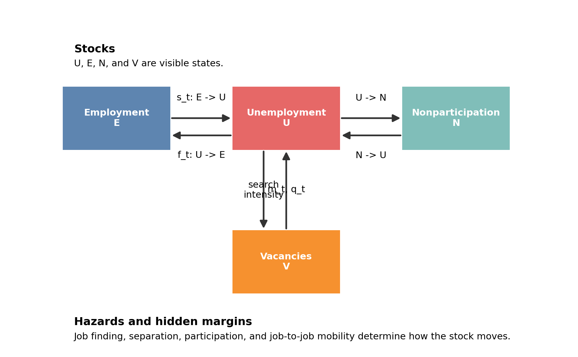
Figure 1:Week 10 organizes aggregate labor adjustment around stocks, hazards, and hidden margins. Unemployment is only one visible outcome; job-to-job transitions, participation shifts, and wage composition matter at the same time.
Figure Figure 1 previews the lecture logic. Aggregate labor adjustment is a map of margins, not a single time series.
Field Core
Stocks, flows, and the law of motion for unemployment
The cleanest opening is the two-state flow benchmark. Let denote unemployment, the employment-to-unemployment hazard, and the unemployment-to-employment hazard. Then unemployment evolves according to
with steady state
Equations (1) and (2) make the first non-negotiable Week 10 point visible. A high unemployment stock can come from high inflows, low outflows, or both. Saying that unemployment rose is therefore not yet an explanation. We need to know which hazard moved and whether the observed stock hides other adjustments in labor-force participation or direct job-to-job mobility Elsby et al., 2009.
The two-state benchmark is useful because it is transparent, but it is not complete. Hidden slack often lives in a three-state system with employment, unemployment, and nonparticipation:
where collects the transition hazards across , , and . The point is not to make the week about participation alone. It is to show where “hidden slack” enters and why a pure unemployment-rate narrative can miss important cyclical movement in labor supply and attachment Krusell et al., 2017.
Matching, tightness, and the Beveridge curve
The canonical matching function is
with market tightness , job-finding rate
and vacancy-filling rate
These equations separate the worker-side and vacancy-side objects. governs the outflow from unemployment; governs recruiting congestion and the expected payoff from vacancy posting. Tightness is therefore good news for workers and bad news for recruiters at the same time. The logic is familiar from Week 4, but Week 10 uses it to study cyclical volatility rather than only steady-state search Shimer, 2005Rogerson et al., 2005.
The reduced-form matching-efficiency residual is
This residual is tempting to call “search efficiency,” but that interpretation requires care. A movement in can reflect changes in search intensity, the mix of workers and vacancies, market segmentation, recruiting effort, or true matching technology. Barnichon and Figura’s central contribution is precisely to show that aggregate matching residuals absorb heterogeneity and composition, not only structural efficiency Barnichon & Figura, 2015. Barlevy, Faberman, Hobijn, and Şahin make the same point in a modern Beveridge-curve context: the reason for an outward shift is historically contingent rather than mechanically tied to one primitive Barlevy et al., 2024.
Under exogenous separation, the steady-state Beveridge object can be written as
Equation (8) is useful because it turns Beveridge-curve interpretation into a decomposition problem. An outward shift can come from weaker tightness, higher separations, lower residual matching efficiency, or a reweighting of searchers and vacancies across segments Elsby et al., 2015.
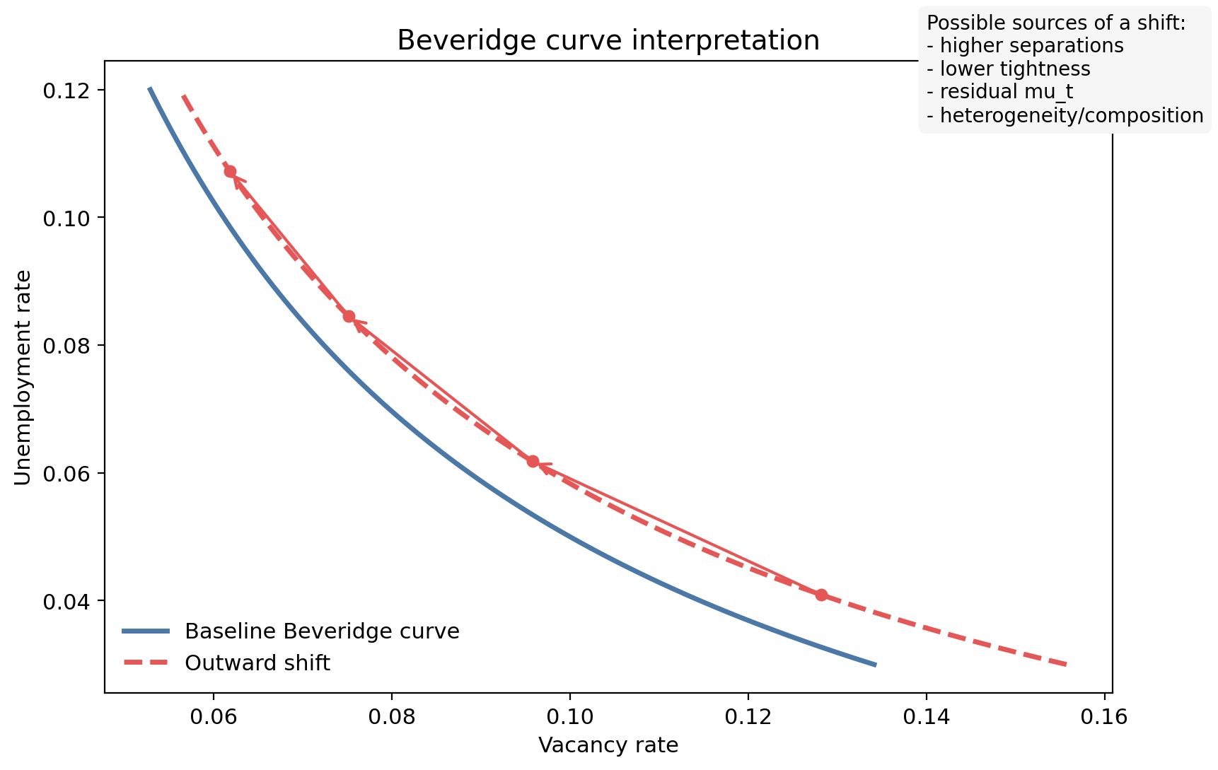
Figure 2:The Beveridge curve is a relationship among unemployment, vacancies, and implied tightness, but shifts in the curve need not identify one single mechanism. Matching residuals mix efficiency, heterogeneity, search intensity, and vacancy composition.
Figure Figure 2 is the lecture’s warning label. A time-series fit to unemployment and vacancies is not the same thing as identification of a labor-market mechanism.
Surplus, vacancy creation, and the volatility puzzle
Search frictions matter for cyclical adjustment because vacancy creation depends on expected surplus. A stripped-down free-entry condition is
where is the vacancy-posting cost and is the value of a filled job to the firm. Match surplus is
where is worker value inside the match and is worker value outside the match. Equations (9) and (10) are the smallest value block that makes the Shimer-Hall debate legible. In the benchmark model, plausible productivity shocks do not move surplus enough to generate the observed volatility of unemployment and vacancies. Shimer’s point is that the canonical model under-amplifies aggregate labor volatility because wages and surplus absorb too much of the shock Shimer, 2005. Hall’s wage-stickiness logic changes that conclusion by keeping wages from moving one-for-one with productivity, which allows surplus and therefore vacancy creation to respond more sharply Hall, 2005.
The labor-economics interpretation matters. This is not primarily a story about inflation. It is a story about how much of an aggregate shock shows up in hiring incentives versus wage adjustment, and therefore about which labor-market margin bears the adjustment.
Table 2:Theory-to-evidence map for aggregate labor-market adjustment
| Theoretical object | Empirical counterpart | Representative paper(s) | Main open question |
|---|---|---|---|
| Matching model and tightness | U, V, job-finding hazard, Beveridge curve | Shimer, 2005; Hall, 2005 | Which primitives generate realistic volatility without breaking wage or flow facts? |
| Stock-flow unemployment accounting | Inflows vs outflows, layoffs vs duration | Elsby et al., 2009 | Which recessions are inflow-driven, outflow-driven, or both? |
| Endogenous separation | E→U hazard, destruction margin | Fujita & Ramey, 2012; Mueller, 2017 | How much of cyclical unemployment is about separations versus hiring? |
| Matching efficiency | Aggregate matching residual, Beveridge shifts | Barnichon & Figura, 2015; Barlevy et al., 2024 | When is a residual really efficiency rather than heterogeneity? |
| Gross worker flows | E/U/N transition system | Krusell et al., 2017 | How important is participation for macro labor adjustment? |
| Job ladder and on-the-job search | E→E hazard, worker reallocation to higher-wage firms | Karahan et al., 2017; Haltiwanger et al., 2018 | How much cyclical adjustment happens through reallocation instead of nonemployment? |
| Wage cyclicality with sorting | Incumbent wages vs mover wages, mismatch-adjusted wage cyclicality | Figueiredo, 2022 | How much measured wage rigidity is really composition or match-quality change? |
Table Table 2 connects these theory objects to the evidence we actually observe. The useful habit is to ask which empirical margin corresponds to the theory object and which important equilibrium object remains latent.
Unemployment stocks versus flows: ins, outs, and what is observed
The stock-flow decomposition literature is valuable because it stops us from treating unemployment as if it moved through one channel. Equation (1) implies that
so cyclical unemployment can be decomposed into an inflow contribution and an outflow contribution around the observed stock. Elsby, Michaels, and Solon show that the relative importance of inflows and outflows changes across recession episodes and horizons. Mild downturns may look mostly like a collapse in job finding; severe downturns often involve both weaker outflows and elevated inflows Elsby et al., 2009.
What is observed in a CPS-style stock-flow decomposition is the transition count or hazard between measured labor-force states. What is inferred is the contribution of those hazards to stock dynamics under a transition-accounting framework. The hidden margin is everything the basic state system does not see directly: recall expectations, misclassification, direct E-to-E mobility, vacancy-side recruiting intensity, and the quality of reemployment matches. That is why national time-series decompositions are indispensable but incomplete.
Separations, endogenous separation, and recessionary unemployment
Week 10 should not treat separation as an exogenous constant. In an endogenous-separation environment, jobs end when match surplus falls below zero for sufficiently weak match quality :
Equivalently,
These expressions convert separation from a nuisance parameter into a labor-market margin that responds to cyclical conditions, heterogeneity, and dispersion in match productivity. Mortensen and Pissarides provide the canonical job-creation and job-destruction framework Mortensen & Pissarides, 1994. Fujita and Ramey show why recession dynamics are often misread if we impose exogenous separations too quickly Fujita & Ramey, 2012. Mueller then sharpens the point by linking separation and cyclical unemployment to sorting across workers and jobs rather than only a representative match Mueller, 2017.
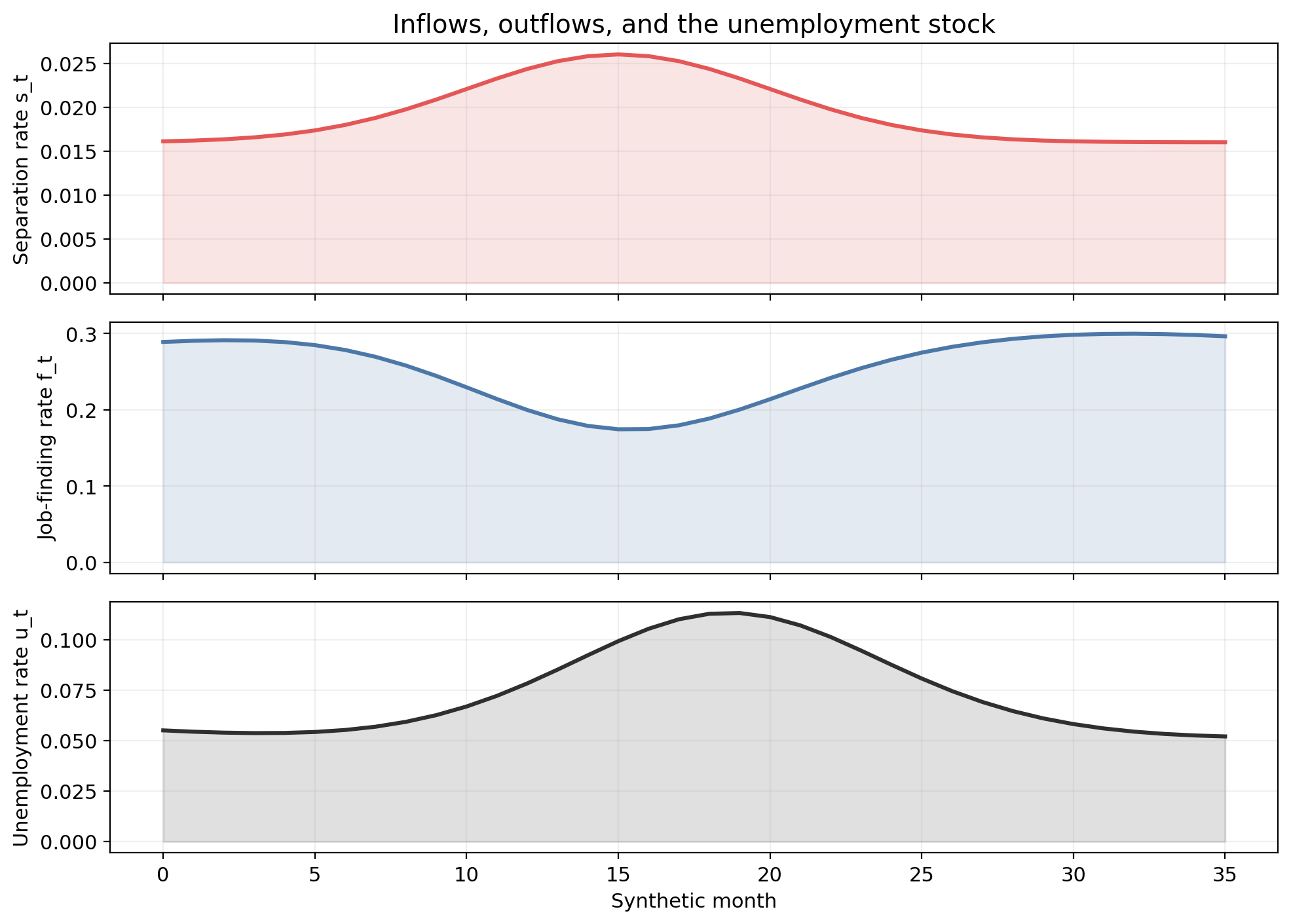
Figure 3:Unemployment dynamics combine inflows, outflows, and endogenous separation. Recessions can raise unemployment because more matches break, because fewer new matches form, or because both forces interact with heterogeneity and recall behavior.
Figure Figure 3 places inflows and outflows on the same visual footing. This is especially important because discussions that overemphasize job finding often understate layoffs, recalls, and the composition of job loss.
Churning is also useful here because not all cyclical worker reallocation appears as net job loss. A compact accounting object is
Equation (14) distinguishes net employment adjustment from replacement hiring and within-firm turnover. In downturns, lower churning may signal weaker replacement hiring and less reallocation even before unemployment peaks. That is one reason aggregate adjustment is not exhausted by the unemployment stock.
Job-to-job transitions, on-the-job search, and cyclical job ladders
Aggregate labor adjustment also runs through employed search and direct job-to-job mobility. A reduced-form on-the-job-search object is
where is the employed offer-arrival rate and the acceptance term captures the chance of receiving a preferable alternative. This makes the core point transparent: the cycle affects wages and mobility not only because unemployed workers find jobs more or less often, but also because employed workers climb job ladders more or less often.
Karahan, Michaels, Pugsley, Şahin, and Schuh show that job-to-job transitions are a first-order source of cyclical wage fluctuations Karahan et al., 2017. Haltiwanger, Hyatt, Kahn, and McEntarfer show that cyclicality in job ladders is organized by firm wage and firm size, which means recessionary adjustment changes who upgrades and which firms receive movers Haltiwanger et al., 2018. The key labor distinction is between aggregate unemployment dynamics and cross-sectional reallocation. Some downturns chiefly destroy hiring and mobility toward better firms; others raise unemployment sharply. Both are labor-market adjustments, but they are not the same object.
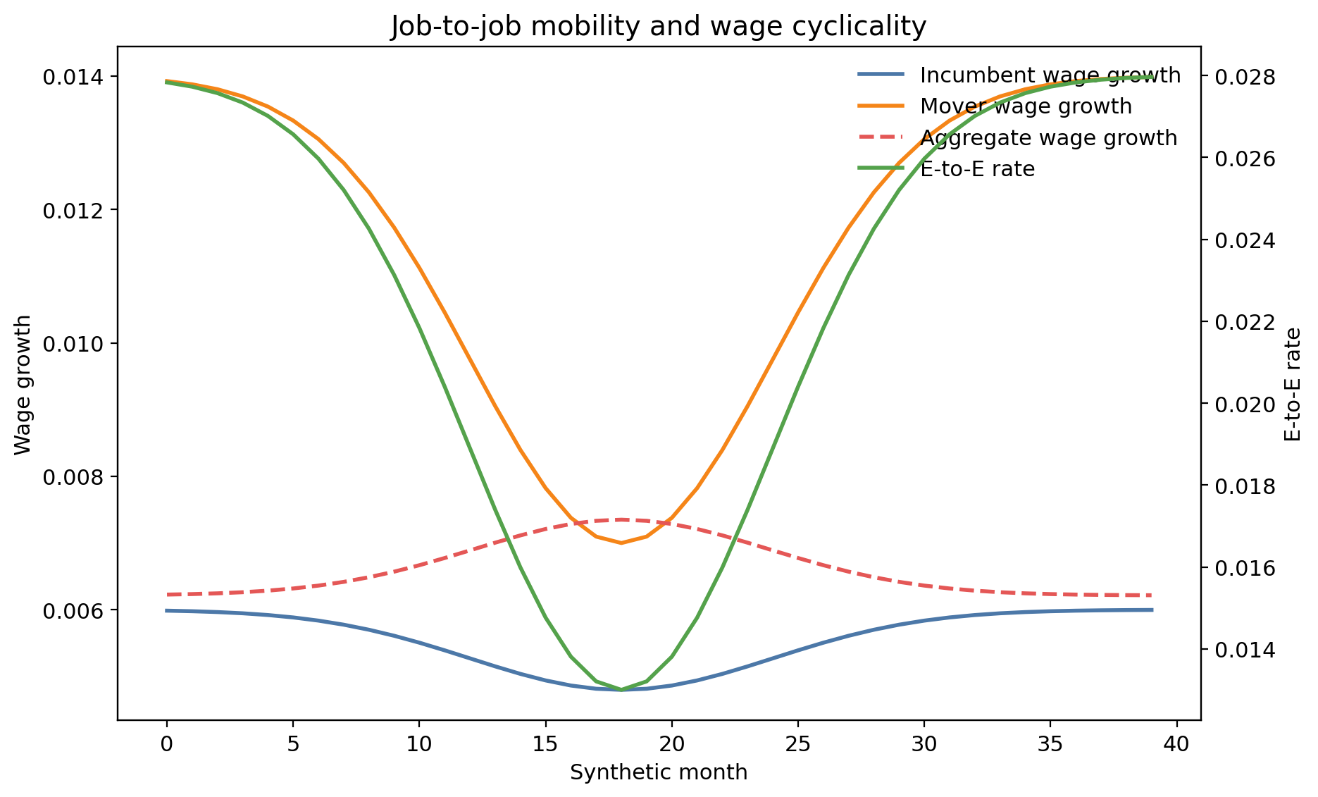
Figure 4:On-the-job search and direct job-to-job mobility connect the business cycle to wage growth and job ladders. A weak labor market compresses outside offers, slows upgrading, and changes who remains in incumbent jobs.
Figure Figure 4 is the bridge from flows to wages. A collapse in can flatten wage growth even before an equivalent movement appears in measured unemployment.
Wages, sorting, and match quality over the cycle
Observed wage cyclicality is hard to interpret because the mean wage mixes incumbent workers, movers, selection into continued employment, and sorting into different firms. A simple decomposition is
where captures incumbent wage cyclicality, captures the wage-growth contribution of job changers and job ladders, and and capture composition and sorting terms. Equation (16) should change how students hear the phrase “wages are weakly cyclical.” That claim may describe true wage rigidity for incumbents, but it may also reflect the collapse of mover wages, the loss of low-wage jobs, or improved average match quality among those who remain employed.
Figueiredo is the key anchor because it shows that measured wage cyclicality is deeply intertwined with labor-market sorting Figueiredo, 2022. Job-ladder evidence reinforces the same lesson: when upward mobility freezes, the observed average wage path need not reveal the true cyclicality of offers or outside options Karahan et al., 2017Haltiwanger et al., 2018.
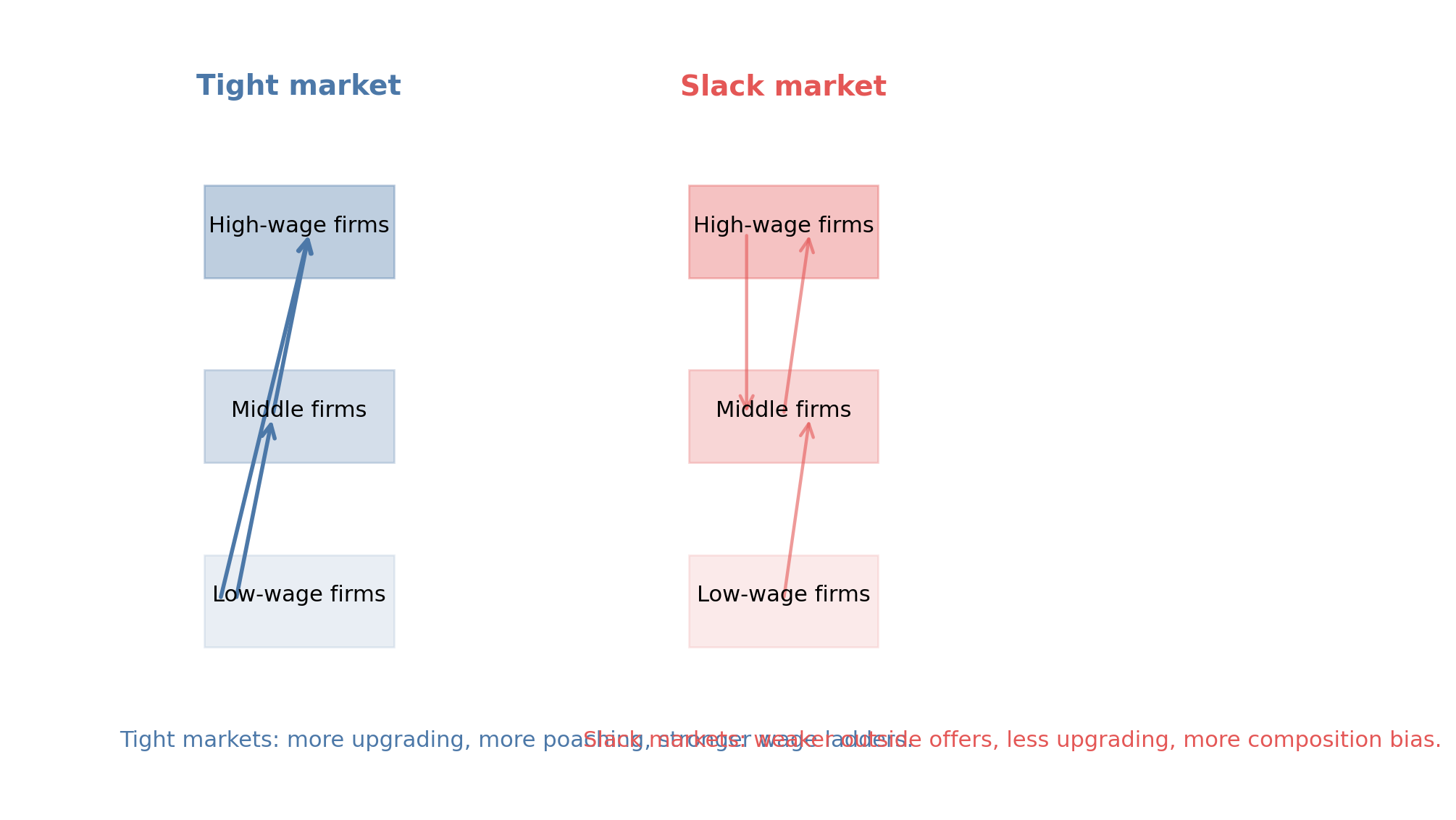
Figure 5:Measured wage cyclicality mixes incumbent wage adjustment, mover wage gains, and changing composition of surviving matches. Cyclical reallocation can make average wages look rigid even when offer distributions and match quality move sharply.
Figure Figure 5 keeps the match-quality and sorting channel explicit. It is the easiest way to show why wage evidence and unemployment evidence need not point to the same margin.
Measurement, identification, and open questions
The right empirical habit in Week 10 is to map each design to its observed and hidden margins.
Table 3:Measurement and identification map for Week 10
| Empirical design / measurement approach | Unit of observation | Margin directly observed | Margin inferred or hidden | Typical strength | Typical limitation |
|---|---|---|---|---|---|
| National Beveridge curve and matching function | Aggregate quarterly or monthly time series | U, V, hires | Matching efficiency / search intensity | Clear macro object, easy replication | Residuals mix efficiency, heterogeneity, and composition |
| Stock-flow decomposition | Aggregate CPS or administrative flows | U→E, E→U, U stock | Relative contribution of inflows vs outflows | Clarifies what drives unemployment changes | Sensitive to classification and transition definitions |
| State or local cyclicality design | State, metro, or region × time | Unemployment, vacancies, wages, E→E rates | How local slack maps into labor-market margins | Useful for quasi-experimental cyclicality comparisons | Local variation may not identify aggregate equilibrium mechanisms |
| Matched employer-employee data | Worker-firm spell | Job-to-job moves, firm wage ladder, separations | Match quality, reallocation, firm-specific adjustment | Rich view of churning and job ladders | Often restricted data and harder to reproduce pedagogically |
| Incumbent vs mover wage measures | Worker-year or worker-quarter | Wage growth by mover status | Wage rigidity vs sorting/composition | Sharp link to wage-setting debates | Wage measures are very composition-sensitive |
| Beveridge-shift decomposition by groups | Labor-market segment × time | Group-specific U and V | Role of heterogeneity / mismatch | Connects efficiency debates to group composition | Requires strong assumptions on segmentation |
Table Table 3 should be read as a design checklist.
National time-series matching and Beveridge-curve evidence uses aggregate monthly or quarterly data. The identifying variation is cyclical movement over time. The unit of observation is the aggregate market-time cell. The observed margins are unemployment, vacancies, hires, and sometimes stock-flow hazards. The hidden margin is the composition of workers and vacancies and the segmentation of search across groups Barnichon & Figura, 2015Elsby et al., 2015.
State and local cyclical designs use differential regional exposure to recessions or demand shifts. The identifying variation is cross-area business-cycle intensity or demand exposure. The unit is the state-year, metro-quarter, or region-time cell. The observed margins may include unemployment, vacancies, wages, or job-to-job mobility. The hidden margin is whether local variation identifies an aggregate equilibrium mechanism or only local relative adjustment.
Matched employer-employee evidence uses worker-firm spells or transitions. The identifying variation comes from cyclical movement across workers, firms, or matched panels. The observed margins are E-to-E moves, wage ladders, separations, and sometimes firm premiums. The hidden margin is the full opportunity set facing the worker and the general-equilibrium vacancy response Haltiwanger et al., 2018Figueiredo, 2022.
The measurement lesson is simple. National time-series evidence is closest to the macro labor object but weak on composition and mechanism. Local variation is often stronger on quasi-experimental design but may miss economy-wide equilibrium. Matched flow evidence is rich on mobility and wage ladders but typically less public and harder to reproduce pedagogically. The research frontier lies in combining these perspectives rather than forcing one design to answer every question Barlevy et al., 2024.
Bridge to Week 11
Week 10 studied cyclical labor-market adjustment: how shocks move unemployment, vacancies, separations, job-to-job mobility, wages, and match quality over the business cycle. Week 11 keeps those margins in view but changes the shock. The transition is from cyclical adjustment to structural adjustment under technology, automation, AI, and labor-demand restructuring. The same labor-market objects remain central; what changes is the persistence and source of the shock.
Research Lab
The Week 10 lab follows the standard Reproduce -> Diagnose -> Transfer structure and is intentionally bounded. The primary anchor is Barnichon & Figura, 2015, where the measured object is an aggregate matching residual rather than an individual worker outcome. The challenge anchor is Elsby et al., 2009, where the central task is to decompose unemployment into inflows and outflows. The optional extension anchor is Karahan et al., 2017, where the margin of interest is job-to-job mobility rather than unemployment itself. The local handout lives at lab.md.
The key research habit is to force the object into the open before discussing results.
What aggregate labor-market object is being measured?
Is the design about stocks, flows, efficiency, wages, or job ladders?
Which margin is observed directly, and which one is inferred?
What cyclical comparison is being made?
Which hidden margin is offstage?
Optional extension block
One extension pushes on Beveridge-curve shifts after 2020. The right question is not whether the Beveridge curve moved, but why: tighter hiring standards, vacancy composition, sectoral reallocation, search intensity, or segmentation Barlevy et al., 2024.
A second extension pushes on job ladders and match quality. The relevant question is whether a weak labor market primarily raises unemployment or instead flattens upward mobility, lowers outside offers, and changes the wage ladder even for those who remain employed Haltiwanger et al., 2018Figueiredo, 2022.
Methods Box
Week 10 only works if the distinctions stay sharp.
Unemployment is a stock; job finding, separation, job-to-job mobility, and participation transitions are hazards.
Job finding, separation, job-to-job transitions, and participation margins are distinct empirical objects and should not be collapsed into a generic notion of “labor-market churn.”
Matching-efficiency residuals are not automatically structural efficiency; heterogeneity, search intensity, vacancy composition, and segmentation can move the same residual.
Cross-sectional reallocation across firms is not the same thing as aggregate unemployment dynamics.
Wage cyclicality for incumbents is not the same object as wage cyclicality for movers.
Measured wage cyclicality is not the same thing as pure wage rigidity once sorting and composition change over the cycle.
National time-series identification, local cyclical variation, and matched employer-employee evidence see different margins and should be treated as complements.
Every empirical claim should name the identifying variation, unit of observation, observed margin, and hidden margin left offstage.
Reading Ladder And References
Ladder A. Canonical framework and the volatility puzzle
Rogerson et al., 2005 for a compact field-course survey of labor-market search models.
Shimer, 2005 for the vacancy-unemployment volatility puzzle in the benchmark model.
Hall, 2005 for wage-stickiness amplification through surplus and vacancy creation.
Ladder B. Flow accounting and Beveridge-curve interpretation
Elsby et al., 2009 for unemployment as an inflow-outflow object.
Elsby et al., 2015 for the Beveridge curve as a labor-market organizing device.
Barnichon & Figura, 2015 for heterogeneity inside aggregate matching residuals.
Ladder C. Separations, reallocation, and job ladders
Mortensen & Pissarides, 1994 for endogenous job creation and destruction.
Fujita & Ramey, 2012 for recession dynamics with endogenous separation.
Mueller, 2017 for separation, sorting, and cyclical unemployment.
Haltiwanger et al., 2018 for cyclical job ladders and E-to-E upgrading.
Ladder D. Wages, job-to-job transitions, and composition
Karahan et al., 2017 for job-to-job transitions as a cyclical wage margin.
Figueiredo, 2022 for wage cyclicality under labor-market sorting.
Barlevy et al., 2024 for recent evidence on why Beveridge-curve shifts differ across eras.
Exercises And Discussion Prompts
Use Equations (1) and (2) to explain how two economies can have the same unemployment rate with different underlying labor-market risks.
Use Equations (4) through (6) to explain why tightness raises the worker-side hazard but lowers the vacancy-side hazard.
Why is Equation (7) not enough to identify a structural matching technology?
Compare the objects in Equations (12) and (15). Which one governs job destruction risk and which one governs job-ladder mobility?
Use Equation (16) to explain how average wage growth can look weakly cyclical even when outside offers are highly cyclical.
Pick one paper from the reading ladder and name its identifying variation, unit of observation, observed margin, and most important hidden margin.
Reproducibility And Code Lab Note
The bounded Week 10 lab is fully local and synthetic. Students first reproduce a Barnichon-Figura-style aggregate matching exercise, then diagnose how much of a Beveridge-style movement is in observed stocks and how much is bundled into an inferred residual, and finally transfer the same reasoning to an Elsby-Michaels-Solon-style stock-flow decomposition and a small synthetic job-to-job cyclicality exercise anchored to Karahan et al., 2017. The point is to make stocks, flows, efficiency residuals, and job ladders explicit without requiring confidential microdata.
Slide Companion Note
The Week 10 slide deck lives at 10
Bridge Forward
Use this closing bridge to carry the module’s labor object, mechanism, and evidence into the next course step or research-design exercise.
- Rogerson, R., Shimer, R., & Wright, R. (2005). Search-Theoretic Models of the Labor Market: A Survey. Journal of Economic Literature, 43(4), 959–988. 10.1257/002205105775362014
- Elsby, M. W. L., Michaels, R., & Ratner, D. (2015). The Beveridge Curve: A Survey. Journal of Economic Literature, 53(3), 571–630. 10.1257/jel.53.3.571
- Elsby, M. W. L., Michaels, R., & Solon, G. (2009). The Ins and Outs of Cyclical Unemployment. American Economic Journal: Macroeconomics, 1(1), 84–110. 10.1257/mac.1.1.84
- Krusell, P., Mukoyama, T., Rogerson, R., & Sahin, A. (2017). Gross Worker Flows over the Business Cycle. American Economic Review, 107(11), 3447–3476. 10.1257/aer.20121662
- Shimer, R. (2005). The Cyclical Behavior of Equilibrium Unemployment and Vacancies. American Economic Review, 95(1), 25–49. 10.1257/0002828053828572
- Barnichon, R., & Figura, A. (2015). Labor Market Heterogeneity and the Aggregate Matching Function. American Economic Journal: Macroeconomics, 7(4), 222–249. 10.1257/mac.20140116
- Barlevy, G., Faberman, R. J., Hobijn, B., & Sahin, A. (2024). The Shifting Reasons for Beveridge Curve Shifts. Journal of Economic Perspectives, 38(2), 83–106. 10.1257/jep.38.2.83
- Hall, R. E. (2005). Employment Fluctuations with Equilibrium Wage Stickiness. American Economic Review, 95(1), 50–65. 10.1257/0002828053828482
- Fujita, S., & Ramey, G. (2012). Exogenous versus Endogenous Separation. American Economic Journal: Macroeconomics, 4(4), 68–93. 10.1257/mac.4.4.68
- Mueller, A. I. (2017). Separations, Sorting, and Cyclical Unemployment. American Economic Review, 107(7), 2081–2107. 10.1257/aer.20121186
- Karahan, F., Michaels, R., Pugsley, B., Sahin, A., & Schuh, R. (2017). Do Job-to-Job Transitions Drive Wage Fluctuations over the Business Cycle? American Economic Review, 107(5), 353–357. 10.1257/aer.p20171076
- Haltiwanger, J. C., Hyatt, H. R., Kahn, L. B., & McEntarfer, E. (2018). Cyclical Job Ladders by Firm Size and Firm Wage. American Economic Journal: Macroeconomics, 10(2), 52–85. 10.1257/mac.20150245
- Figueiredo, A. (2022). Wage Cyclicality and Labor Market Sorting. American Economic Review: Insights, 4(4), 425–442. 10.1257/aeri.20210161
- Mortensen, D. T., & Pissarides, C. A. (1994). Job Creation and Job Destruction in the Theory of Unemployment. Review of Economic Studies, 61(3), 397–415. 10.2307/2297896