Monopsony, Measurement, and Sources of Power
Learning Objectives
By the end of Week 6, students should be able to:
define monopsony as employer wage-setting power rather than only as a one-firm market structure;
distinguish classic one-firm monopsony, oligopsony, and modern dynamic/search monopsony;
explain why labor supply to the firm is not the same object as market labor supply;
connect finite labor-supply elasticity to the firm to marginal labor cost and wage markdowns;
separate markdowns, firm wage premia, rent-sharing, and concentration proxies;
explain why employer concentration is not the same thing as monopsony, even when it is informative;
evaluate empirical papers by naming the identifying variation, the unit of observation, the observed margin, and the key unobserved object;
organize the leading sources of monopsony power and connect them to the policy block that begins in Week 7.
Opening Orientation
The economic question for Week 6 is the natural sequel to Week 5: once wages are set by posting, bargaining, or internal wage rules rather than by a frictionless spot market, when do firms actually possess enough wage-setting power that the monopsony lens becomes the right way to organize theory and evidence Robinson, 1933Manning, 2021Sokolova & Sorensen, 2021?
Bridge
Week 5 taught students that a meeting technology is not enough. Search frictions, outside options, and internal wage rules all matter for pay because they determine the protocol that maps surplus into wages. Week 6 asks the next question: how much power does the employer have inside that protocol? A posted wage can still face a highly elastic labor supply to the firm, or it can face a much less elastic one. A bargained wage can still be disciplined by strong outside options, or it can be bargained in an environment where worker mobility is weak.
That is why Week 6 is not a separate detour. It is the conduct environment for Week 5. Wage posting, bargaining, pass-through, and firm wage premia are easier to interpret once we know whether labor supply to the firm is close to perfectly elastic or instead meaningfully downward sloping. The forward bridge is equally important. If firms possess wage-setting power, then minimum wages, noncompetes, transparency rules, merger scrutiny, and worker-protection institutions can have very different implications than under the competitive benchmark. That is why Week 7 turns explicitly toward policy incidence.
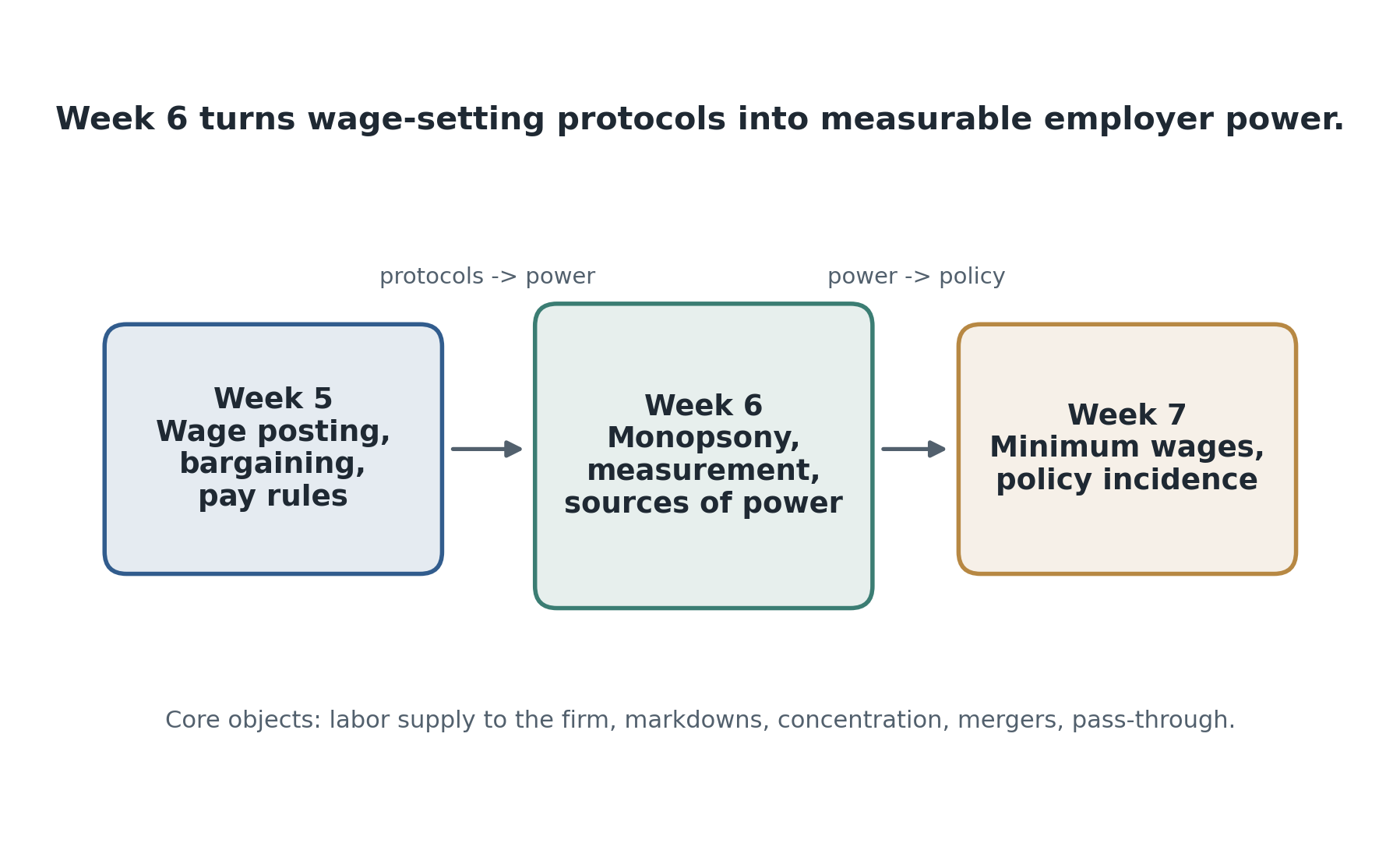
Figure 1:Week 6 sits between wage-setting protocols and the policy block. It turns Week 5’s protocols into measurable employer wage-setting power and then hands those objects to Week 7.
Figure Figure 1 is the course repositioning map for the week. The point is not that every labor market is a company town. The point is that employer power is best studied as a spectrum of wage-setting power generated by frictions, differentiation, and market structure Manning, 2021Ashenfelter et al., 2022.
Why monopsony is the natural sequel to Week 5
Week 5 already broke the frictionless benchmark by showing that wages may be posted, bargained, or administratively constrained. But those protocol labels alone do not tell us how responsive employment is to a firm’s own wage or how much a firm can mark wages below worker marginal revenue product. Week 6 therefore makes five transitions explicit.
from wage-setting protocol to wage-setting power;
from outside options to labor supply to the firm;
from search frictions to modern dynamic monopsony;
from wage pass-through evidence to monopoly-style wedge objects such as markdowns;
from positive wage-setting theory to later policy design.
Table 1:Monopsony concepts and measurement objects
| Object | What it means | Typical empirical proxy or design | Key caution |
|---|---|---|---|
| Classic monopsony | One dominant employer faces upward-sloping labor supply and chooses wage/employment jointly | Textbook benchmark; occasionally useful for intuition in thin local markets | Too stark for many modern labor markets |
| Dynamic/search monopsony | Firms have wage-setting power because workers move across jobs slowly and outside options are imperfect | Search models, quit elasticities, offer arrival rates, job ladders | Power can exist even with many firms |
| Labor supply to the firm | Elasticity of a firm’s employment or applicant flow with respect to its own wage | Wage variation, online markets, applications data, dual-jobholder settings | Different margins can produce different elasticities |
| Markdown | Gap between marginal revenue product of labor and wage | Production-side estimation, matched employer--employee data | Requires stronger structure and harder-to-observe objects |
| Concentration | Market-share or HHI proxy for employer dominance | Commuting zone × occupation concentration, merger shocks | Not a structural measure of power on its own |
| Firm wage premium | Persistent firm-specific pay component after worker controls | AKM-style wage decompositions | Not all firm wage premia reflect monopsony |
| Rent-sharing / pass-through | Wage response to firm or outside-option shocks | Firm-shock designs, bargaining/pass-through designs | Can arise under multiple wage-setting models |
Table Table 1 is the opening taxonomy. It is useful because it says plainly which objects are primitives, which are structural wedges, which are reduced-form statistics, and which are proxies.
Field Core
What monopsony is and is not
The clean definition for Labor II is this: monopsony is employer wage-setting power, meaning the firm faces an upward-sloping labor supply curve and therefore cannot hire an additional worker without affecting the wage or worker flow it must offer Robinson, 1933Manning, 2021. That definition is broader and more useful than the textbook image of a single employer in an isolated town.
Classic monopsony remains a valuable benchmark because it makes the logic transparent. The firm chooses wage and employment jointly because labor supply to the firm is upward sloping. But modern labor economics rarely treats this textbook case as the full empirical description. Workers search while employed, jobs differ in amenities and rules, information is incomplete, and mobility across firms is costly or slow. Wage-setting power can therefore arise even with many firms, provided workers do not move frictionlessly across all alternatives Manning, 2021Sokolova & Sorensen, 2021.
The practical lesson is that monopsony is better treated as a spectrum than as a binary market structure. Employer size is not identical to employer power. Local concentration is not identical to employer power. A firm may operate in a market with many establishments yet still face a finite labor-supply elasticity because workers perceive jobs as differentiated or because search and switching are costly. Conversely, concentration can be high in a narrow measured market even when workers possess wider effective outside options than the researcher can see.
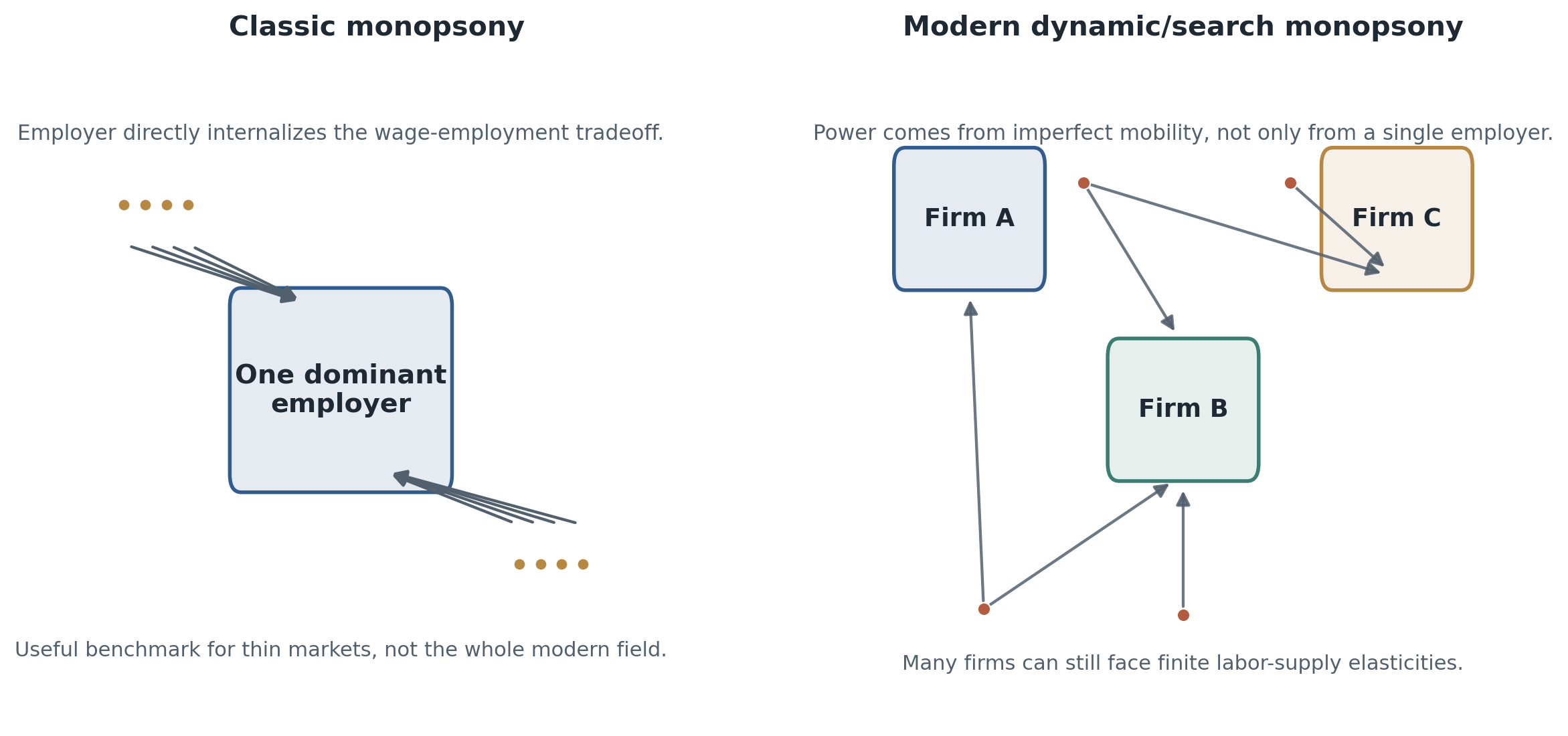
Figure 2:Classic monopsony is a sharp one-buyer benchmark. Modern monopsony allows wage-setting power to arise from frictions and differentiation even with many firms.
Figure Figure 2 is the first major conceptual split of the week. The left panel is the classic benchmark. The right panel is the modern search-based or dynamic interpretation in which wage-setting power is compatible with multiple firms and ongoing worker mobility.
Labor supply to the firm is not market labor supply
The central theoretical object is labor supply to the firm:
Equation (1) is deliberately local. It asks how a firm’s own employment responds to its own wage . This is not the same object as the market labor supply elasticity, which asks how total labor supplied to an entire market responds to the market wage. A firm can face a finite elasticity even if aggregate labor supply is quite elastic, because workers are reallocating across firms rather than deciding whether to work at all Manning, 2021Sokolova & Sorensen, 2021.
This distinction matters because many empirical designs do not observe total labor-force entry or exit. They observe applications, vacancies, separations, quits, employment-to-employment flows, or retention. Those are firm-level mobility margins. They tell us how strongly a worker’s own-firm choice responds to changes in wage offers, amenities, and outside options.
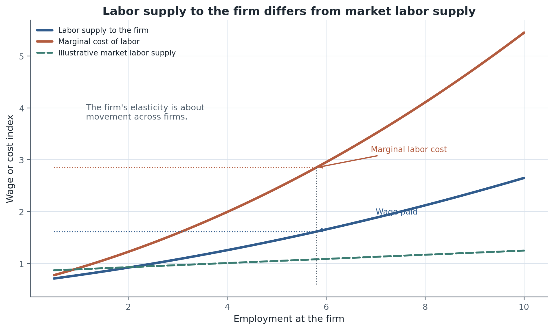
Figure 3:The relevant elasticity for monopsony is labor supply to the firm. Marginal labor cost lies above the wage schedule when the firm’s labor supply is finite.
Figure Figure 3 makes the distinction visual. The firm’s labor supply curve is upward sloping, and the marginal cost of labor lies above the wage schedule because expanding employment requires the firm to improve pay or recruiting conditions on infra-marginal workers as well.
Marginal labor cost and markdowns
Once labor supply to the firm is finite, the firm pays a marginal labor cost above the wage:
Equation (2) is the compact wedge object students should remember. When is very large, marginal labor cost approaches the wage and the competitive benchmark reappears. When the elasticity is moderate, the cost of adding a worker exceeds the posted wage because the firm must move along an upward-sloping supply curve.
The empirical counterpart often highlighted in modern papers is the markdown:
where is the worker’s marginal revenue product of labor. Equation (3) summarizes the wedge between what the worker contributes at the margin and what the worker is paid. A markdown greater than one is consistent with labor market power, but it is not the same object as a firm wage premium or a rent-sharing elasticity Berger et al., 2022Yeh et al., 2022.
This separation is essential. Markdown estimates are production-side wedge objects. Firm wage premia are persistent pay components estimated from worker-firm wage panels. Rent-sharing or pass-through estimates ask how wages respond to changes in firm-side or outside-option shocks. These objects may all point toward labor market power, but they are not numerically interchangeable and need not agree even in the same sector.
Why concentration is not the same thing as monopsony
Concentration remains useful because thin labor markets and large employers can weaken competitive pressure, but concentration is at most a proxy:
Equation (4) measures concentration through market shares in market . It is useful because concentration is often observable in local occupation-by-geography cells when direct wage-setting wedges are not. But concentration is not itself a structural measure of wage-setting power.
There are at least three reasons the proxy can mislead. First, measured markets may not equal workers’ effective opportunity sets. Second, job differentiation and amenities can generate monopsony even in unconcentrated settings. Third, concentration can move wages through channels that do not map one-to-one into a single labor-supply elasticity or markdown. This is exactly why the literature increasingly pairs concentration evidence with wage variation, merger evidence, or production-side wedges rather than treating concentration as sufficient on its own Azar et al., 2019Prager & Schmitt, 2021Jarosch et al., 2024.
How the literature measures monopsony power
The most useful organizing principle is by measurement object rather than by paper chronology.
Table 2:Measurement and identification map for monopsony
| Approach | Unit of observation | Identifying variation | What it identifies best | Main limitation |
|---|---|---|---|---|
| Applications or task-level wage variation | Vacancy, task, or requester | Within-platform or experimental wage changes | Recruiting / labor-supply elasticity to firm | Often narrow setting; external validity |
| Quit / separation elasticity methods | Worker--firm spell | Wage differences and mobility hazards | Dynamic monopsony through retention margins | Sensitive to job-ladder structure and unobserved offers |
| Production-side markdown estimation | Plant or firm | Production and wage moments plus structure | Wedge between MRPL and wages | Requires strong assumptions and rich data |
| Concentration proxies | Local market or market-year | Cross-market concentration differences | Descriptive link between structure and wages | Concentration may proxy power poorly |
| Merger or consolidation designs | Market, hospital, firm, occupation | Quasi-experimental shifts in employer concentration | Causal wage effect of market-structure change | Sector-specific and partial-equilibrium |
| Firm-shock / pass-through designs | Worker--firm panel | Product demand or tax shocks | Wage sensitivity to firm-side shocks | Maps imperfectly into a single monopsony parameter |
Table Table 2 is the empirical backbone for the week. It groups designs into labor-supply elasticity designs, retention or quit elasticity designs, markdown estimation, concentration proxies, merger studies, and pass-through approaches.
Labor-supply and recruiting elasticities
The cleanest direct object is labor supply to the firm or a closely related recruiting elasticity. Dube et al., 2020 is the ideal field-core anchor because wage variation is unusually clean in an online labor market. The identifying variation is within-platform wage posting or experimental wage differences. The observed unit is the task, applicant pool, or requester-task cell. The observed margin is recruiting intensity or staffing probability. The unobserved object is how that elasticity maps to broader labor market behavior outside the platform. The design therefore identifies a firm-facing labor-supply object very well, but in a narrow institutional environment.
Quit and separation elasticity approaches observe worker-firm spells rather than vacancy-task cells. The identifying variation is wage differences across otherwise similar jobs or firms. The observed margins are retention, separations, or employment-to-employment flows. The unobserved object is the full job-ladder structure, including offers the researcher never sees. These methods are often the most direct bridge between search models and modern monopsony because they treat worker mobility as the source of employer power Manning, 2021Sokolova & Sorensen, 2021.
Production-side markdowns
Production-side methods use plant or firm production moments to recover the wedge between wages and marginal revenue product. Yeh et al., 2022 is the core challenge paper for this week because it forces students to distinguish a production-side markdown object from a recruiting elasticity. The identifying variation comes from observed production and compensation moments under additional structure. The unit of observation is the plant or firm. The observed margin is the relationship among labor shares, revenue productivity, and wages. The key unobserved object is the true marginal revenue product and the validity of the production structure used to infer it.
Markdown estimates can therefore be economically large even when reduced-form concentration or pass-through estimates look more modest. That is not necessarily a contradiction. The methods are using different observed margins, different units, and different latent objects.
Concentration proxies and market-structure shocks
Concentration designs observe market-level structure and link it to wages or mobility. Azar et al., 2019 is central because it shows how concentration proxies and direct labor-supply objects can be read together rather than as substitutes. The identifying variation is cross-market employer concentration. The unit is a local labor market, often geography by occupation. The observed margin is wage level or wage growth. The key unobserved object is whether the measured market coincides with worker substitution possibilities.
Merger or consolidation designs sharpen the causal claim by using quasi-experimental shifts in employer structure:
Equation (5) is intentionally reduced-form. It captures the idea that wages may change when measured market structure changes, but it does not by itself identify the full underlying monopsony wedge. Prager & Schmitt, 2021 is the flagship design here. The identifying variation is hospital mergers that change employer concentration. The unit is the market or worker-market setting. The observed margin is wage change after consolidation. The key unobserved object is how fully the merger-induced wage effect maps to a deeper labor-supply or markdown parameter.
Firm shocks and pass-through
Pass-through and firm-shock approaches sit at the boundary between Week 5 and Week 6. Berger et al., 2022 and related work use firm-side shocks or labor share moments to infer labor market power from wage responses or allocative wedges. The identifying variation can be firm demand, productivity, or tax changes. The observed unit is a worker-firm panel or firm panel. The observed margin is wage pass-through or dispersion in wages and employment. The unobserved object is how much of that pass-through reflects bargaining, sorting, or monopsonistic conduct. These approaches are powerful precisely because they force students to keep wage-setting protocol and labor-market-power objects conceptually distinct.
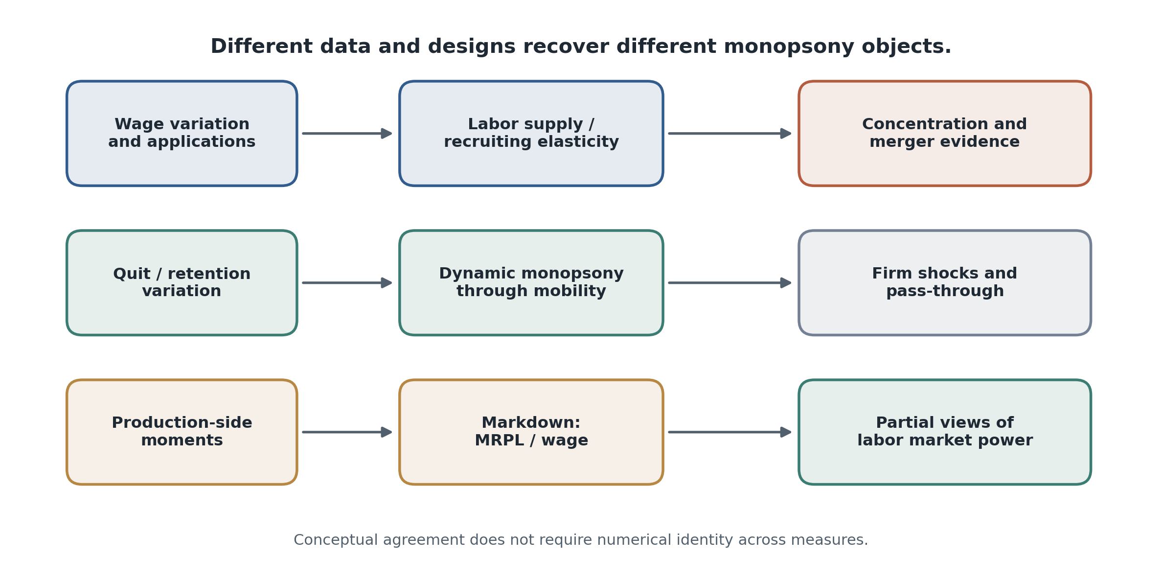
Figure 4:Different empirical designs observe different margins and therefore identify different monopsony objects. The numbers need not line up exactly to tell a coherent conceptual story.
Figure Figure 4 shows why the literature can produce different estimates without genuine contradiction. A recruiting elasticity, a quit elasticity, a markdown, a concentration coefficient, and a merger effect all illuminate monopsony, but they illuminate different slices of it.
Sources of monopsony power
Table 3:Sources of monopsony power
| Source of power | Mechanism | Canonical implication | Example empirical setting |
|---|---|---|---|
| Search and mobility frictions | Workers do not instantaneously find or move to best alternatives | Finite labor-supply elasticity to each firm | Job ladders, quit hazards, unemployment-to-job flows |
| Job differentiation and amenities | Jobs differ in schedule, safety, prestige, flexibility, location, and internal rules | Workers tolerate wage gaps to obtain valued nonwage attributes | Teachers, hospitals, remote work, public-sector jobs |
| Information frictions / wage opacity | Workers do not fully observe wages or alternatives | Outside options are weaker than observed nominal competition suggests | Online markets, salary-history settings, transparency reforms |
| Geographic and occupational immobility | Workers are locally or skill constrained | Thin markets amplify employer power | Rural labor markets, healthcare, specialized occupations |
| Concentration and employer size asymmetry | Large employers internalize less competitive pressure | Wages fall after consolidation or in highly concentrated markets | Hospital mergers, local occupation markets |
| Contractual or institutional barriers | Noncompetes, visa restrictions, licensing, pension lock-in | Switching costs rise and outside options weaken | Healthcare, guest workers, public pensions |
| Internal wage rules | Firms constrain wage competition through grades, schedules, or administrative pay | Market shocks pass through incompletely to wages | Large organizations, public-sector pay, internal labor markets |
Table Table 3 is the week’s source taxonomy. The main point is that modern monopsony research increasingly treats employer power as arising from overlapping sources rather than from one mechanism alone.
Search and mobility frictions remain the foundational source. Workers do not instantly observe or accept the best alternative, and on-the-job search takes time. Amenities and job differentiation matter because workers trade wages against schedule flexibility, safety, prestige, mission, remote work options, and internal rules. Information frictions matter because nominally available outside options may not be salient or credible to workers. Geographic and occupational immobility matter because specialized or thin markets can leave workers with few realistic substitutes. Concentration and employer size asymmetry matter because large employers can internalize some of the wage consequences of their hiring behavior. Contractual and institutional barriers matter because noncompetes, licensing, immigration restrictions, or pension lock-in raise switching costs. Internal wage rules matter because a firm may dampen market pressure through salary bands, grades, or administrative pay practices even in settings with many outside employers.
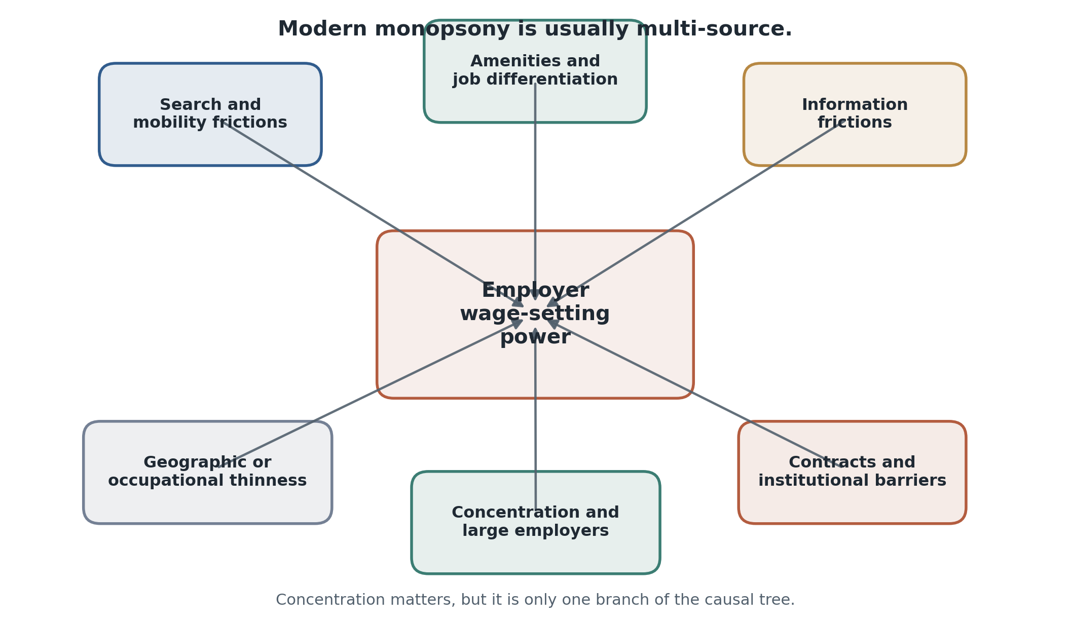
Figure 5:Modern monopsony is usually multi-source. Frictions, preferences, information, concentration, and institutional barriers can all contribute to the same observed wage-setting power.
Figure Figure 5 is deliberately broad because the empirical literature now treats monopsony as a bundle of mechanisms. This is also why concentration is informative but incomplete. Concentration captures one possible source of power. It does not exhaust the concept.
Empirical designs and flagship papers: what they identify
The best way to teach the empirical literature is to require four sentences for every paper:
what is the identifying variation;
what is the observed unit;
what observed margin is measured;
what important monopsony object remains unobserved.
Dube et al., 2020 uses direct wage variation in an online labor platform. The unit is the task or task-requester cell. The measured margin is applications or fill probability. The unobserved object is how that platform elasticity generalizes to off-platform mobility, amenities, and longer-run equilibrium adjustment.
Yeh et al., 2022 uses production-side moments in a matched employer setting. The unit is the plant or firm. The measured margin is the wedge between wages and inferred marginal revenue product. The unobserved object is the true production structure, the correct marginal product mapping, and any dynamic mobility margins not directly seen in the production-side object.
Prager & Schmitt, 2021 uses merger-induced changes in concentration. The unit is the hospital labor market or worker-market environment. The measured margin is post-merger wage change. The unobserved object is the full general-equilibrium response, including worker resorting and any nonwage adjustments.
Azar et al., 2019 uses cross-market concentration. The unit is a local labor market cell. The measured margin is wage differences across concentration environments. The unobserved object is the correct labor market boundary and any omitted amenity or product-market differences correlated with concentration.
Berger et al., 2022 asks how labor market power reshapes wages, allocations, and welfare in a more structural equilibrium framework. The identifying variation is broader because the paper combines theory and data moments rather than leaning on one reduced-form shock. The observed unit is firm or market aggregates together with wage objects. The unobserved object is any single sufficient statistic for monopsony, which is precisely why structural synthesis is attractive and difficult.
Frontier extension block: unresolved measurement issues
This week should end with a substantial extension block rather than a short appendix. Four unresolved issues are especially productive.
First, concentration can misclassify true labor market power when market boundaries are coarse, workers search across occupation-geography cells, or amenities create differentiation that is not visible in market shares. Second, markdown measurement outside manufacturing remains hard because marginal revenue products are even less directly observed in services, healthcare, and remote platform settings. Third, amenities and compensating differentials complicate measurement because high-wage firms may also offer valued nonwage attributes, making observed mobility responses hard to interpret. Fourth, new administrative, vacancy, and platform datasets promise cleaner wage variation and worker-flow measurement, but they do not automatically solve the problem of defining the relevant outside option set Manning, 2021Jarosch et al., 2024.
This extension block is also where the bridge to inequality and sorting should be made explicit. Monopsony can amplify wage dispersion not only by lowering the overall wage level relative to marginal product, but also by interacting with worker heterogeneity, amenities, and firm wage policies. That is one reason the frontier increasingly links labor market power to firm heterogeneity, worker sorting, and policy design Berger et al., 2022Ashenfelter et al., 2022.
Research Lab
The Week 6 lab is built around Reproduce -> Diagnose -> Transfer.
The reproduction anchor is Dube et al., 2020. Students work with a bounded synthetic online-task setting where the wage varies cleanly and the observable outcome is recruiting intensity. The goal is to make the labor-supply-to-the-firm elasticity concrete rather than abstract.
The diagnose anchor is Yeh et al., 2022. Students then confront a different monopsony object: the markdown. The lab asks them to say plainly why a production-side markdown object is not the same as a recruiting elasticity, what identifying structure is added, and what remains latent.
The transfer and optional extension anchor is Prager & Schmitt, 2021. Students move to a stylized employer concentration or merger panel and ask what a reduced-form wage response to changing market structure does and does not identify. The local handout lives at lab.md.
Methods Box
Week 6 only works if eight distinctions remain explicit.
Labor supply to the firm versus market labor supply: monopsony is about the elasticity facing the firm, not only labor-force participation at the market level.
Classic static monopsony versus dynamic/search monopsony: the former is a benchmark, the latter is the modern field-core framework.
Markdowns versus firm wage premia versus rent-sharing: these are related but non-identical wage-setting objects.
Concentration proxies versus causal evidence on market power: concentration is descriptive unless paired with stronger design or structure.
Sources of power rooted in frictions and preferences versus sources rooted in employer concentration: modern monopsony often combines both.
Reduced-form merger or policy evidence versus structural measurement: both are informative, but they answer different questions.
Evidence without design language is not enough: every result in this week should name the identifying variation, the unit of observation, the observed margin, and the key unobserved object.
Different monopsony measures need not agree numerically: disagreement in magnitudes can arise because the methods target different margins, time horizons, and latent wedges.
Reading Ladder And References
Required / field core
Robinson, 1933 for the classic benchmark and the original wage-setting-power logic.
Manning, 2021 for the modern conceptual map from classic monopsony to dynamic labor market power.
Sokolova & Sorensen, 2021 for a field-wide synthesis of labor-supply elasticity evidence.
Dube et al., 2020 for a direct labor-supply-to-the-firm design with clean wage variation.
Yeh et al., 2022 for production-side markdown measurement.
Strong empirical complements
Azar et al., 2019 for the relationship between concentration proxies and other monopsony measures.
Prager & Schmitt, 2021 for causal evidence from employer consolidation.
Berger et al., 2022 for structural equilibrium labor market power.
Optional / frontier / synthesis
Jarosch et al., 2024 for granular search and market structure in modern labor markets.
Ashenfelter et al., 2022 for synthesis and policy-facing takeaways from the modern empirical literature.
Exercises And Discussion Prompts
Use Equation (1) to explain why a firm can face monopsonistic labor supply even when market labor supply is fairly elastic.
Compare Equations (2) and (3). Which one is a labor-cost object and which one is a wage-productivity wedge?
Why does high concentration in Equation (4) not by itself prove monopsony?
In Dube et al., 2020, what varies, what unit is observed, what margin is observed, and what key object remains latent?
In Yeh et al., 2022, why can a markdown estimate move differently from a recruiting elasticity estimate without contradiction?
In Prager & Schmitt, 2021, what does a wage response to consolidation identify well, and what deeper labor-market-power object remains only partially identified?
Use Table Table 3 to propose two markets with similar concentration but different sources of monopsony power.
Why is it useful to teach monopsony as a spectrum of wage-setting power rather than as a binary “competitive versus one-employer” classification?
Propose one transfer design using public vacancy data, a stylized concentration panel, or a simulated plant markdown panel. Name the observed unit, observed margin, identifying variation, and the key unobserved object.
Reproducibility And Code Lab Note
The Week 6 code lab is deliberately bounded and local. The reproduction step uses a synthetic online-task dataset inspired by Dube et al., 2020 to estimate a labor-supply-to-the-firm object from direct wage variation. The diagnose step uses a synthetic plant panel inspired by Yeh et al., 2022 to force a comparison between recruiting elasticities and markdowns. The transfer step uses a synthetic concentration-and-merger panel in the spirit of Prager & Schmitt, 2021 so students can see what a reduced-form structure shock identifies and what it does not. The bounded path runs locally without confidential microdata; the local handout lives at lab.md.
Slide Companion Note
The slide deck at 06
Bridge Forward
Use this closing bridge to carry the module’s labor object, mechanism, and evidence into the next course step or research-design exercise.
- Robinson, J. (1933). The Economics of Imperfect Competition. Macmillan.
- Manning, A. (2021). Monopsony in Labor Markets: A Review. ILR Review, 74(1), 3–26. 10.1177/0019793920922499
- Sokolova, A., & Sorensen, T. (2021). Monopsony in Labor Markets: A Meta-Analysis. ILR Review, 74(1), 27–55. 10.1177/0019793920965562
- Ashenfelter, O., Card, D., Farber, H. S., & Ransom, M. R. (2022). Monopsony in the Labor Market: New Empirical Results and New Public Policies. Journal of Human Resources, 57(S), S1–S10. 10.3368/jhr.monopsony.57.S.S1
- Berger, D., Herkenhoff, K., & Mongey, S. (2022). Labor Market Power. American Economic Review, 112(4), 1147–1193. 10.1257/aer.20191521
- Yeh, C., Macaluso, C., & Hershbein, B. (2022). Monopsony in the U.S. Labor Market. American Economic Review, 112(7), 2099–2138. 10.1257/aer.20200025
- Azar, J., Marinescu, I., & Steinbaum, M. (2019). Measuring Labor Market Power Two Ways. AEA Papers and Proceedings, 109, 317–321. 10.1257/pandp.20191068
- Prager, E., & Schmitt, M. (2021). Employer Consolidation and Wages: Evidence from Hospitals. American Economic Review, 111(2), 397–427. 10.1257/aer.20190690
- Jarosch, G., Nimczik, J. S., & Sorkin, I. (2024). Granular Search, Market Structure, and Wages. Review of Economic Studies, 91(6), 3569–3607. 10.1093/restud/rdae004
- Dube, A., Jacobs, J., Naidu, S., & Suri, S. (2020). Monopsony in Online Labor Markets. American Economic Review: Insights, 2(1), 33–46. 10.1257/aeri.20180150