Labor Demand and Production

Learning Objectives¶

By the end of Week 1, students should be able to:

write down a static production problem and explain why labor demand is a derived demand rather than a primitive object;
solve a cost-minimization problem and distinguish the production function, cost function, conditional factor demand, and total labor demand;
derive the scale and substitution components of an own-wage response and connect them to the Hicks--Marshall laws of derived demand;
distinguish conditional from total labor demand, and short-run from long-run elasticities, without sliding into dynamic adjustment or monopsony;
map payroll-tax reforms, city-industry demand shocks, product-market cost shocks, and matched employer-employee rent-sharing designs into the margin each design identifies;
connect static labor demand back to Labor I’s worker-side objects and forward to Week 2 on adjustment costs.

Opening Orientation¶

The economic question for the opening week of Labor II is direct: once firms transform inputs into output, how do wages, technology, factor substitution, labor’s cost share, and product demand determine how much labor they want to hire?

Bridge¶

Labor I mostly asked how workers choose, invest, sort, and respond to policy. Labor II begins by re-centering the same observed outcomes inside the firm’s problem. Employment, hours, and wages still matter, but now they appear as objects pinned down by production, cost minimization, output demand, and later by frictions and institutions. The opening move is therefore a reorientation rather than a reset.

The static benchmark is intentionally narrow. This week does not yet study why firms adjust slowly, how wages are bargained, or when firms have labor market power. Those belong to Weeks 2, 5, and 6. Week 1 instead asks where the firm would like to be after a shock if it could move immediately.

The primitive object is the technology:

q = F(L,K;A),

(1)

where $L$ is labor, $K$ is a second input, and $A$ indexes productivity. Equation (1) is the bridge from Labor I to Labor II. Workers supplied labor in Labor I; firms now demand it because labor helps produce marketable output. Derived demand means labor demand cannot be interpreted without saying what technology looks like, what the firm can substitute toward, and how the product market absorbs cost shocks Hicks, 1932Hamermesh, 1993.

The static benchmark already explains why this week matters for policy. Payroll taxes change labor costs, product-demand expansions change the scale of production, and technology changes can alter both marginal products and substitution possibilities. Later weeks will add wage-setting, search, bargaining, and institutions, but those mechanisms all sit on top of the benchmark derived-demand logic rather than replacing it.

Field Core¶

Production, marginal products, and the static firm problem¶

The simplest competitive benchmark says the firm hires labor until the value of the marginal product equals the wage:

p\frac{\partial F(L,K;A)}{\partial L} = w.

(2)

Equation (2) is useful because it keeps the economic objects in view. A higher product price $p$ or higher productivity $A$ raises the value of labor’s marginal product. A higher wage $w$ raises the marginal cost of labor. But this condition alone hides a key distinction: some comparative statics hold output fixed and isolate substitution across inputs, while others allow output itself to move.

That distinction is why the chapter spends time on cost minimization rather than treating the first-order condition as the whole story. Empirically, many designs observe a wage or cost shock and then record employment responses after output has adjusted. Theory has to tell us when that observed response is a substitution object, when it is a scale object, and when it is both.

Cost minimization and conditional labor demand¶

Start with the dual problem:

\min_{L,K} \; wL + rK \quad \text{s.t.} \quad F(L,K;A) \ge q.

(3)

Holding output $q$ fixed gives conditional factor demand. The Lagrangian for Equation (3) implies

\frac{F_L(L,K;A)}{F_K(L,K;A)} = \frac{w}{r},

(4)

so the cost-minimizing input mix equates the marginal rate of technical substitution to the relative factor price. Equation (4) is the clean substitution object: output is fixed, so the firm is only rearranging inputs while delivering the same $q$ .

For a constant-returns technology with elasticity of substitution $\sigma$ , the own-wage elasticity of conditional labor demand is

\eta^{c}_{LL} = \frac{\partial \ln L^{c}(q,w,r;A)}{\partial \ln w}\Big|_{q} = -(1-s_L)\sigma,

(5)

where $s_L$ is labor’s cost share. Equation (5) is the core substitution result. Conditional demand becomes more elastic when labor is easier to substitute away from and less elastic when labor already absorbs most of total cost. Nothing in this object yet says how much output the firm sells.

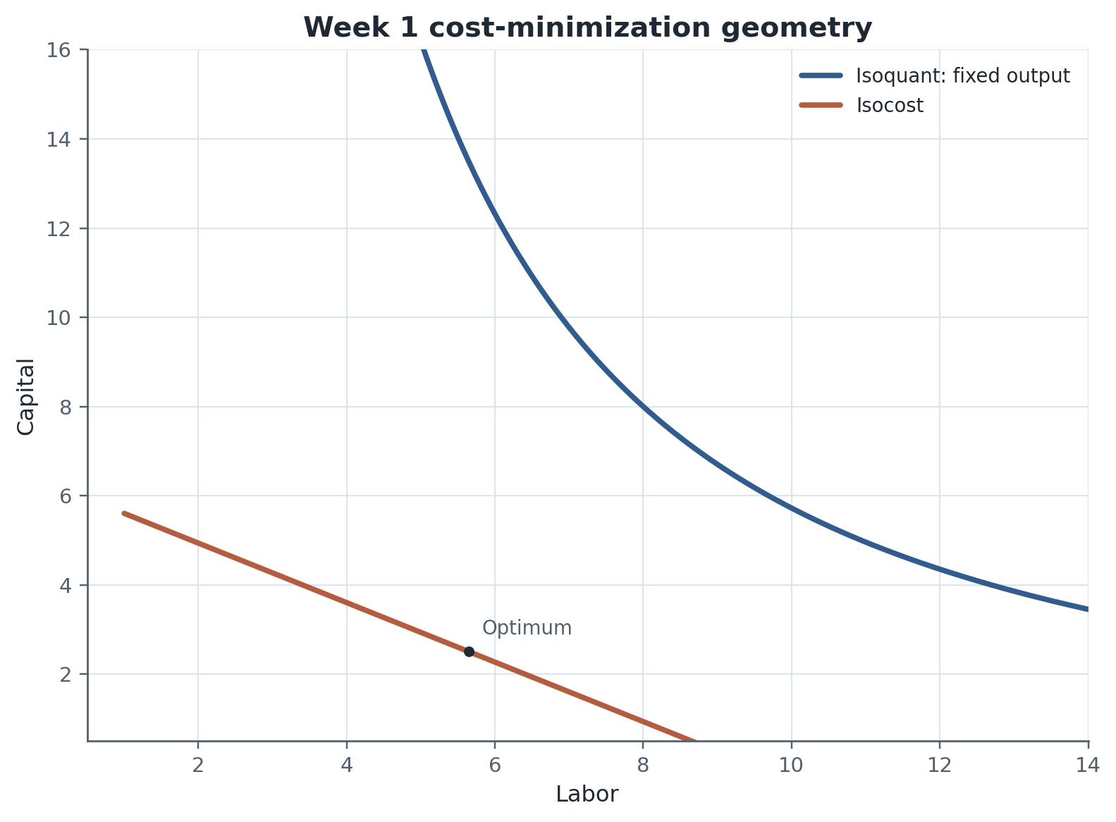
Isoquant-isocost geometry for Week 1. The tangency illustrates Equation : holding output fixed, conditional labor demand isolates substitution across inputs rather than the full employment response to a wage or tax shock. — Figure 1:Isoquant-isocost geometry for Week 1. The tangency illustrates Equation (4): holding output fixed, conditional labor demand isolates substitution across inputs rather than the full employment response to a wage or tax shock.

Figure Figure 1 is therefore not decorative micro theory. It is the cleanest way to see why conditional labor demand is not yet the incidence object students often want in applied work. When a policy changes wages or payroll taxes, the firm rarely holds output fixed in the data.

From conditional to total labor demand¶

Total labor demand lets output move:

\frac{d\ln L}{d\ln w} = \underbrace{\frac{\partial \ln L^{c}}{\partial \ln w}\Big|_{q}}_{\text{substitution}} + \underbrace{\frac{\partial \ln L}{\partial \ln q}\frac{d\ln q}{d\ln w}}_{\text{scale}}.

(6)

Equation (6) is the scale/substitution decomposition. The first term is the same fixed-output re-optimization from Equation (5). The second term says that a higher wage raises marginal cost, reduces desired output when product demand is downward sloping, and therefore lowers labor demand even if the firm would not substitute much toward capital.

Under constant returns and an isoelastic product-demand schedule with absolute elasticity $\eta$ , the decomposition becomes

\eta_{LL} = \frac{d\ln L}{d\ln w} = -(1-s_L)\sigma - s_L\eta.

(7)

Equation (7) is the compact static benchmark for the rest of the week. The own-wage elasticity of total labor demand is more negative when substitution is easier and when product demand is more elastic. The scale effect loads on labor’s cost share because the output contraction matters more when labor is a large component of marginal cost.

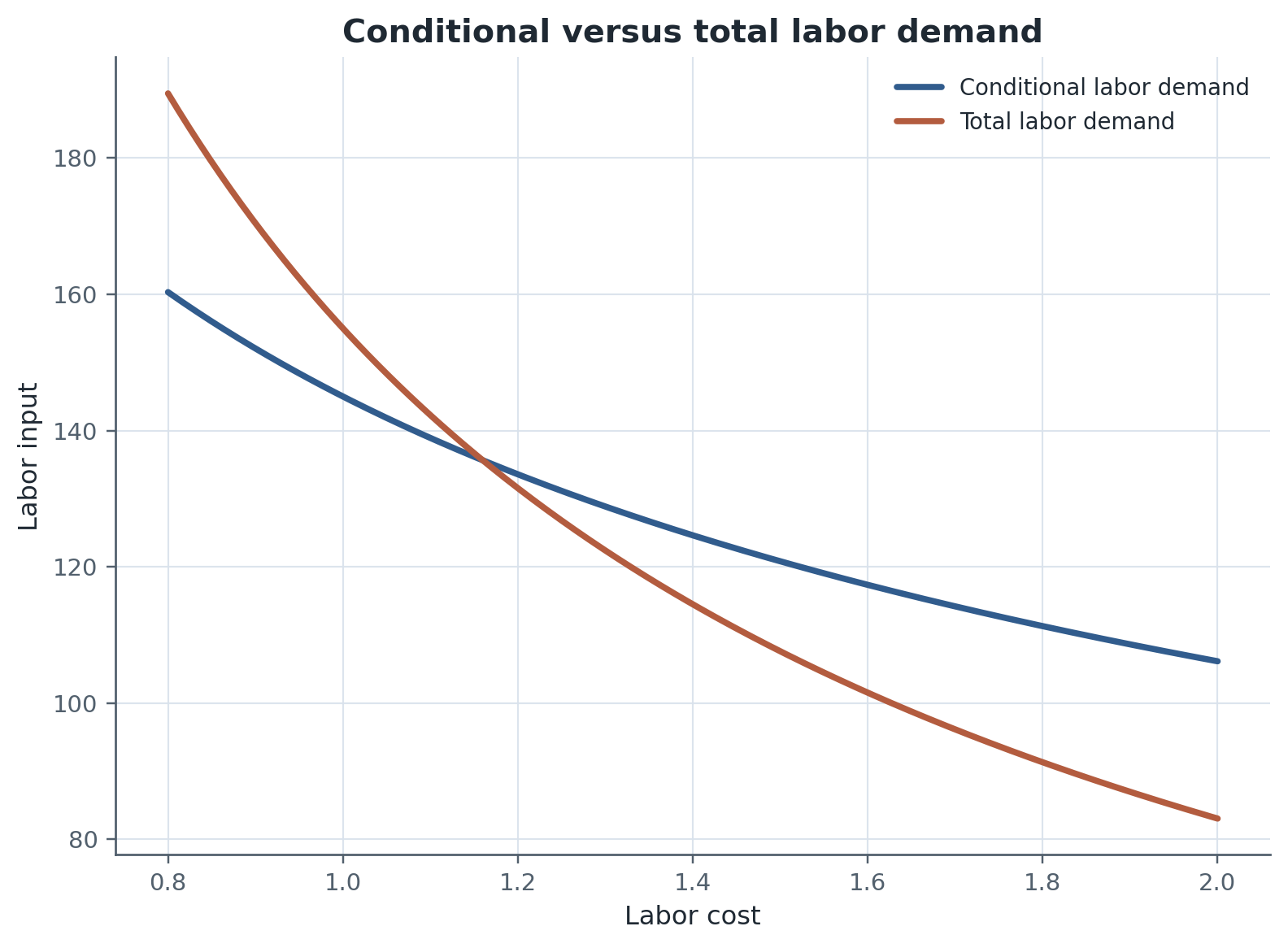
Conditional and total labor demand in the same diagram. The total curve is more elastic because it combines within-firm substitution with the output contraction summarized by Equation . — Figure 2:Conditional and total labor demand in the same diagram. The total curve is more elastic because it combines within-firm substitution with the output contraction summarized by Equation (6).

Figure Figure 2 is the quickest way to translate the theory into empirical caution. A design that mostly reveals substitution with output fixed is not estimating the same object as a design in which prices, output, and employment all adjust together.

Hicks--Marshall laws in plain language¶

The Hicks--Marshall laws of derived demand summarize the logic of Equation (7) Hicks, 1932Hamermesh, 1993.

Labor demand is more elastic when labor can be substituted away from more easily.
Labor demand is more elastic when product demand is more elastic.
Labor demand is more elastic when labor accounts for a larger share of total cost.
Labor demand is more elastic when the supply of other factors is more elastic, because substitution margins are easier to use in practice.

The first three laws are visible directly in Equation (7). The fourth is a useful reminder that “capital” is not always a frictionless margin. When capital, tasks, or organizational choices are effectively fixed, even a textbook static model can look more inelastic over short horizons.

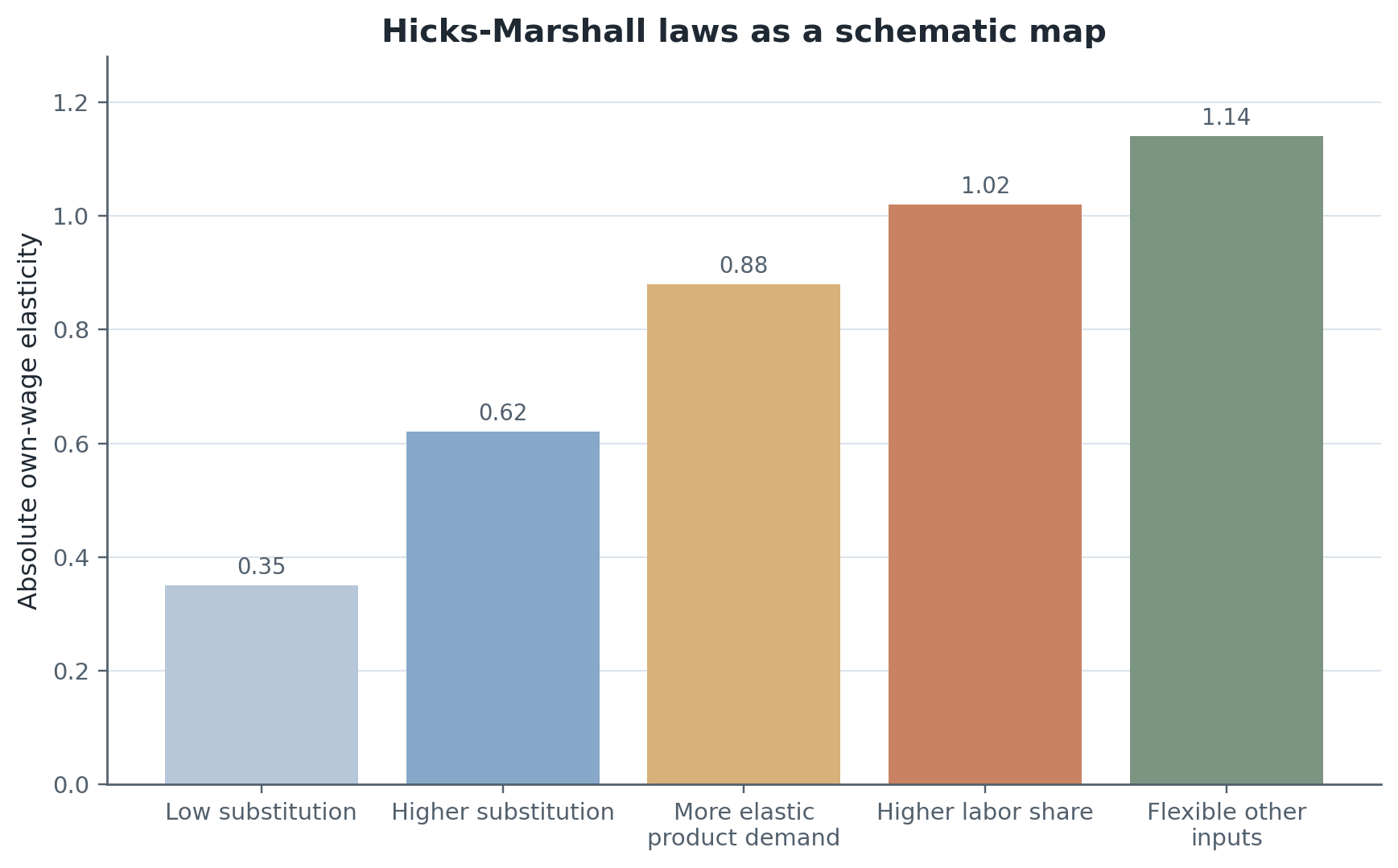
Figure 3:Schematic Hicks--Marshall map. The figure emphasizes that substitution possibilities, product-demand elasticity, labor’s cost share, and the flexibility of other inputs all shape the absolute magnitude of labor-demand elasticities.

Figure Figure 3 is also the bridge from blackboard theory to policy interpretation. It explains why the same payroll-tax cut can look modest in one sector and large in another, and why product-market structure belongs inside labor-demand reasoning rather than in a later footnote.

Short run versus long run inside a static benchmark¶

Students often hear “static” and infer “single horizon.” That is too coarse. Even in a one-period comparative statics lecture, the effective horizon changes with which inputs are treated as flexible. If capital is quasi-fixed, the firm moves mainly along a short-run labor-demand schedule. If capital, tasks, or organizational form can adjust, the long-run schedule is more elastic because more substitution margins open up.

This is the simplest clean way to distinguish short-run from long-run elasticities without formally introducing adjustment costs yet. The theory is static, but the empirical object depends on whether the observed window is next quarter, next year, or several years after a reform. That is why Week 2 matters: it will turn the statement “firms do not get to their long-run target immediately” into an explicit dynamic problem.

Table 1:Labor-demand elasticity taxonomy for Week 1

Object	What is held fixed?	Main economic content	Typical source of variation	Why it matters
Conditional labor demand	Output	Substitution across inputs	Factor-price variation in a cost-minimization frame	Cleanest route to substitution elasticities
Total labor demand	Nothing on output	Substitution plus scale/output response	Wage, tax, or cost shocks with output adjustment	Relevant for employment incidence
Short-run labor demand	Some capital or organization fixed	Limited substitution margins	Very near-term shocks	Often less elastic
Long-run labor demand	More inputs variable	Broader substitution and reorganization	Persistent shocks or long panels	Usually more elastic
Own-wage elasticity	Other prices fixed	Response of labor to labor cost	Wage or payroll-tax shocks	Central labor-demand object
Cross-price elasticity	Labor price fixed	Co-movement with capital/other inputs	Capital-cost or task-price changes	Reveals substitutability/complementarity
Labor demand under rent sharing / wage-setting	Employment and wages may both move	Demand interacts with surplus division	Profit or tax shocks with wage responses	Foreshadows Weeks 5--6

Table Table 1 should be read as a translation device. Conditional versus total demand, short-run versus long-run demand, and own- versus cross-price objects are not competing labels for one number. They are different economic objects that answer different policy questions.

Empirical labor-demand designs: what do they identify?¶

Modern labor-demand papers are best organized by identifying variation rather than chronology.

Table 2:Empirical design map for static labor demand

Design bucket	Typical variation	Margin observed	Object most closely identified	Representative anchor
Payroll-tax reform	Exogenous change in labor cost	Employment, wages, hiring, incidence	Total labor demand and incidence	Saez et al., 2019
City-industry demand shift	Local or sectoral demand shock	Employment and wages across places/sectors	Labor demand elasticity with equilibrium spillovers	Beaudry et al., 2018
Product-market cost shock	Excise/sales-tax or input-cost change	Prices, employment, wages, pass-through	Product-demand link to labor demand	Butters et al., 2022
Rent-sharing / profit shock	Firm profitability or rents	Wages, employment, worker-firm outcomes	Boundary between demand and wage-setting	Card et al., 2018

Payroll-tax or labor-cost reforms vary the firm’s effective wage bill directly. The observed margins are employment, hiring, hours, and wages, so these designs speak to total labor demand and economic incidence rather than to conditional substitution alone Saez et al., 2019. The main limitation is that wage-setting and institutional responses can share the stage with pure derived demand.

City-industry demand shocks move labor demand from the revenue side. The observed margins are employment and wages across local labor markets, often with equilibrium spillovers across places or sectors. This is the clearest Week 1 bridge to why local labor-demand estimates are not purely partial equilibrium objects Beaudry et al., 2018. The identifying variation is not a change in the wage paid by one firm; it is a demand shift that changes firms’ desired scale.

Product-market cost shocks ask whether firms facing local or sector-specific marginal-cost changes absorb the shock through prices, quantities, wages, or some combination Butters et al., 2022. These designs identify the product-market side of labor demand: if prices adjust strongly, the scale effect on employment may be muted. If prices adjust weakly, employment may carry more of the incidence.

Matched employer-employee rent-sharing designs sit at the boundary between labor demand and wage-setting. Variation in firm profitability or rents is linked to wages and worker-firm outcomes, not just to headcount. The observed object is therefore not a pure own-wage labor-demand elasticity. It is evidence about how firm-level rents transmit into wage inequality and surplus sharing Card et al., 2018. That is why Week 1 can preview later wage-setting weeks without collapsing into them.

Static labor demand and policy incidence¶

A payroll tax inserts a wedge between the worker’s wage and the firm’s effective labor cost:

c_L = (1+\tau)w.

(8)

Equation (8) is the clean Week 1 policy object. Statutory incidence says who remits the tax. Economic incidence asks who ultimately absorbs it through wages, employment, prices, or profits. In the pure static benchmark, the employment response is larger when total labor demand is elastic. In later weeks, wage-setting, bargaining, and labor market power will change how much of the wedge shows up in wages versus employment.

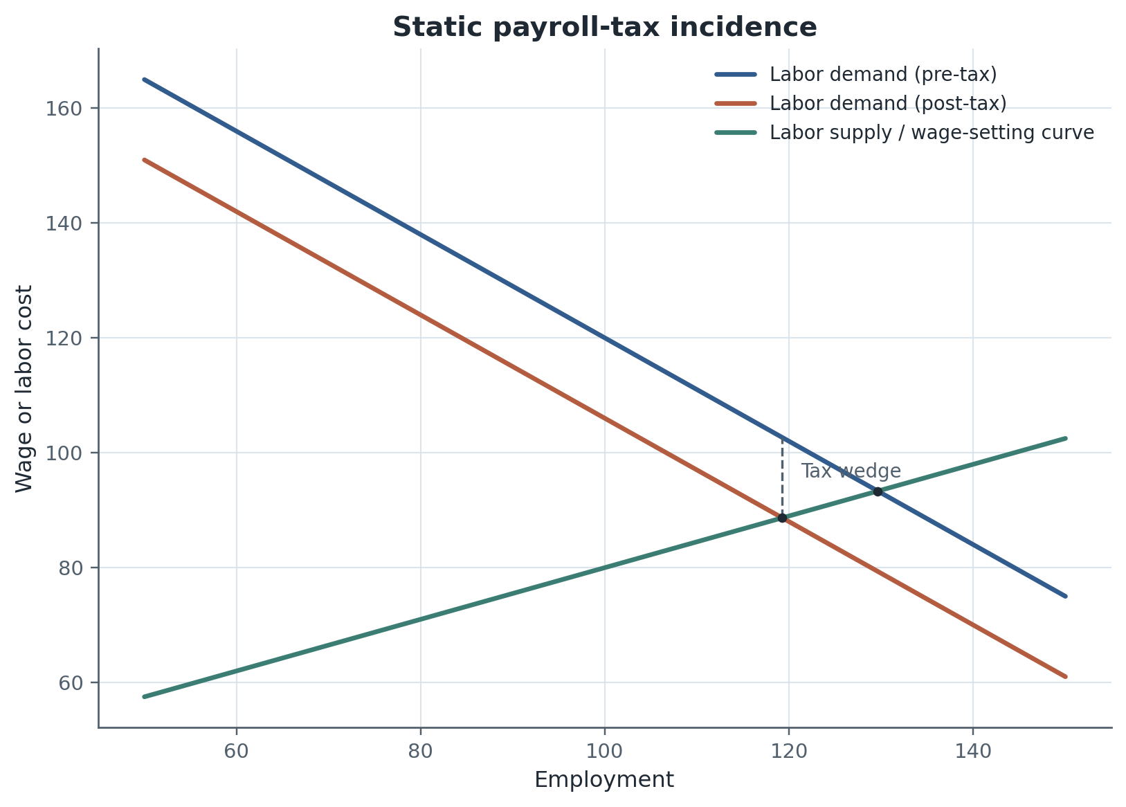
Figure 4:Static payroll-tax incidence schematic. The tax creates a wedge between worker wages and employer labor cost; the employment response depends on the total labor-demand elasticity and, beyond the benchmark, on wage-setting and labor-supply conditions.

Figure Figure 4 keeps the logic disciplined. Payroll taxes and labor-cost reforms are not special topics. They are the most immediate application of the derived-demand framework because they move the firm’s effective labor cost directly.

Table 3:Static-demand policy and incidence map

Shock or policy	First margin hit	Key comparative-static question	Main Labor II connection
Payroll tax cut	Effective labor cost	How much appears in employment vs wages?	Week 5 wage-setting; Week 6 monopsony
Wage subsidy	Labor cost net of subsidy	Does hiring expand more than wages?	Worker-targeted vs firm-targeted policy comparison
Product-demand expansion	Revenue side / scale	How much does labor demand shift via output?	Week 10 technology and Week 11 trade shocks
Capital-cost change	Relative factor price	Are labor and capital substitutes or complements?	Week 2 dynamic adjustment
Local cost shock	Marginal cost and pricing	Do product markets mute or amplify labor responses?	Firm heterogeneity and institutional pass-through

Table Table 3 emphasizes what should be asked every time a policy or cost shock appears: which margin is hit first, what comparative-static object is relevant, and whether the shock mostly reveals substitution, scale, or later-week wage-setting mechanisms.

Bridge to Week 2¶

Week 1 tells us where the firm wants to be after a shock. Week 2 asks why it often does not get there immediately. Once hiring, firing, training, and reorganization are costly, observed employment paths reflect both the static target from Equation (7) and the speed with which firms can approach that target.

Research Lab¶

The main research lesson from Week 1 is that “the labor-demand elasticity” is rarely a single transportable number. What is identified depends on the source of variation, the time horizon, the observed margin, and the product-market environment. A payroll-tax estimate, a city-industry demand-shift estimate, and a matched employer-employee rent-sharing estimate can all be valuable while speaking to different pieces of the labor-demand system.

Week 1 also previews why firm heterogeneity matters. Firms with different cost shares, market power, product-demand elasticities, or task technologies need not have the same labor-demand response even within the same broad industry. That is one reason modern labor-demand work often looks like firm heterogeneity plus product-market structure rather than a single aggregate elasticity exercise.

Optional extension block¶

An optional extension can go in either of two directions.

The first is rent sharing. Card et al., 2018 is a useful bridge because it shows how firm-specific rents map into wage inequality. That evidence sits at the boundary between pure derived demand and wage-setting, which makes it a natural preview of Weeks 5 and 6.

The second is product-market pass-through. Butters et al., 2022 is a useful extension because it shows why local cost shocks need not translate one-for-one into local employment changes when multi-market or national firms can absorb shocks through broader pricing and production margins.

Methods Box¶

Week 1 uses one discipline repeatedly: name the variation, then name the margin.

Conditional labor demand holds output fixed and isolates substitution across inputs.
Total labor demand lets output move and therefore combines substitution and scale.
Short-run elasticities keep some inputs or organizational choices effectively fixed; long-run elasticities allow more margins to adjust.
Payroll-tax and labor-cost reforms move effective labor cost directly and are often read through incidence.
City-industry demand shocks move desired scale and therefore identify total demand with local-equilibrium spillovers.
Product-market cost shocks reveal whether prices, output, and employment absorb the shock.
Matched employer-employee rent-sharing designs track wages and firm rents, so they often sit at the boundary between labor demand and wage-setting.

The practical rule is simple: do not report an empirical result without naming the identifying variation and the margin observed.

Reading Ladder And References¶

Bridge¶

Hicks, 1932 for the original derived-demand logic and the language behind the Hicks--Marshall laws.
Hamermesh, 1993 for the canonical labor-demand benchmark and the cleanest field-style treatment of elasticities.

Field Core¶

Beaudry et al., 2018 for a modern city-industry labor-demand design that emphasizes local demand variation and equilibrium spillovers.
Saez et al., 2019 for payroll-tax incidence, labor-cost wedges, and the link from static demand to wage-setting.
Acemoglu & Autor, 2011 for the broader technology, task, and substitution perspective that places Week 1 inside contemporary labor economics.

Research Lab¶

Butters et al., 2022 for product-market absorption of local cost shocks.
Card et al., 2018 for firm rents, wage inequality, and the boundary between derived demand and surplus sharing.

Exercises And Discussion Prompts¶

Use Equations (5) and (7) to explain why a payroll-tax estimate is not automatically a conditional labor-demand estimate.
In Figure Figure 2, what empirical design would come closest to tracing the conditional curve rather than the total curve?
Why does a high labor share magnify policy incidence in Equation (7) even when the elasticity of substitution is unchanged?
Beaudry, Green, and Sand and Saez, Schoefer, and Seim both study labor demand, but their identifying variation is different. Which margin is most naturally observed in each case?
How would a strong matched employer-employee rent-sharing result change the way you interpret a simple static labor-demand benchmark?

Reproducibility And Code Lab Note¶

The Week 1 lab follows the standard Reproduce -> Diagnose -> Transfer workflow. The bounded reproduction path uses a local synthetic city-industry panel inspired by Beaudry et al., 2018 so students can estimate a compact labor-demand relationship without confidential microdata. The diagnose step asks students to say clearly which object the local-demand design identifies and which margins it misses. The transfer step then uses a stylized payroll-tax scenario file to compare conditional and total labor-demand logic, with Saez et al., 2019 as the challenge anchor and Butters et al., 2022 as the optional extension on product-market absorption. The local handout lives at lab.md.

Slide Companion Note¶

The slide deck at 01-labor-demand-and-production.tex should stay sharper than the chapter: central question, Labor I to Labor II bridge, the static firm problem, cost minimization, the scale/substitution decomposition, Hicks--Marshall laws, payroll-tax incidence, empirical design buckets, and the bridge to Week 2 on dynamic adjustment.

Bridge Forward¶

Use this closing bridge to carry the module’s labor object, mechanism, and evidence into the next course step or research-design exercise.

References¶

Hicks, J. R. (1932). The Theory of Wages. Macmillan.
Hamermesh, D. S. (1993). Labor Demand. Princeton University Press.
Saez, E., Schoefer, B., & Seim, D. (2019). Payroll Taxes, Firm Behavior, and Rent Sharing: Evidence from a Young Workers’ Tax Cut in Sweden. American Economic Review, 109(5), 1717–1763. 10.1257/aer.20171937
Beaudry, P., Green, D. A., & Sand, B. M. (2018). In Search of Labor Demand. American Economic Review, 108(9), 2714–2757. 10.1257/aer.20141374
Butters, R. A., Sacks, D. W., & Seo, B. (2022). How Do National Firms Respond to Local Cost Shocks? American Economic Review, 112(5), 1737–1772. 10.1257/aer.20201524
Card, D., Cardoso, A. R., Heining, J., & Kline, P. (2018). Firms and Labor Market Inequality: Evidence and Some Theory. Journal of Labor Economics, 36(S1), S13–S70. 10.1086/694153
Acemoglu, D., & Autor, D. H. (2011). Skills, Tasks and Technologies: Implications for Employment and Earnings. In O. Ashenfelter & D. Card (Eds.), Handbook of Labor Economics (Vol. 4B, pp. 1043–1171). Elsevier. 10.1016/S0169-7218(11)02410-5