Wage Determination and Returns to Skill
Learning Objectives
By the end of Week 5, students should be able to:
distinguish wages, earnings, hourly pay, lifetime earnings, productivity, and rents;
write down and interpret a Mincer-style wage equation and explain why it is a benchmark rather than a complete causal model;
explain why schooling premia are shaped by selection, comparative advantage, and heterogeneous returns;
distinguish descriptive OLS returns, IV/LATE-style returns, average treatment effects, and marginal policy effects;
explain how worker sorting across firms or places changes the interpretation of observed returns to schooling;
connect Week 5 wage-measurement discipline to Week 6 household decisions and Week 8 inequality decompositions;
map empirical designs to estimands, not just to identification slogans.
Opening Orientation
The economic question for the week is direct: if Week 4 treated skill as an accumulated state variable, how do labor markets translate that state into observed pay, and what exactly is being measured when an empirical paper reports a “return to schooling” or a “return to skill” Mincer, 1974Card, 1999Heckman et al., 2006?
Bridge
Week 4 built the supply side of productive capacity. Workers invested in schooling, training, and earlier-life environments, and those investments changed the latent skill stock that later shows up in market outcomes. Week 5 asks what happens at the pricing stage. Observed wages are not direct readouts of productivity. They combine productive capacity, the market price of skill, hours, compensating differentials, access to better-paying jobs, and sometimes rents Roy, 1951Mincer, 1974Willis & Rosen, 1979.
That distinction matters immediately. A wage premium for college is not automatically a pure return to human capital. It may partly reflect who selects into college, which firms hire college workers, which cities reward skill more steeply, and which jobs bundle better amenities with lower or higher pay Card, 1999Card et al., 2018Diamond, 2016. The recurring Week 5 question is therefore not “is the coefficient positive?” but “what object does this estimate actually recover?”
The Mincer benchmark and what it buys us
The canonical organizing benchmark is the Mincer wage equation:
where is hourly wage, is schooling, and is potential experience. Equation (1) is useful because it turns a complicated wage-setting problem into a disciplined descriptive map: level differences, experience slopes, and lifecycle concavity can all be summarized in one compact object Mincer, 1974Heckman et al., 2006.
But Equation (1) does not interpret itself. The coefficient is a descriptive schooling premium unless stronger assumptions make it causal. Even in the cleanest case, it is a return to measured schooling in wages, not necessarily a return to latent skill. And once the outcome becomes annual earnings rather than hourly pay, hours decisions are folded into the coefficient as well. That is why Week 2 labor supply, Week 4 human capital, and Week 5 wage determination belong in sequence rather than in isolation.
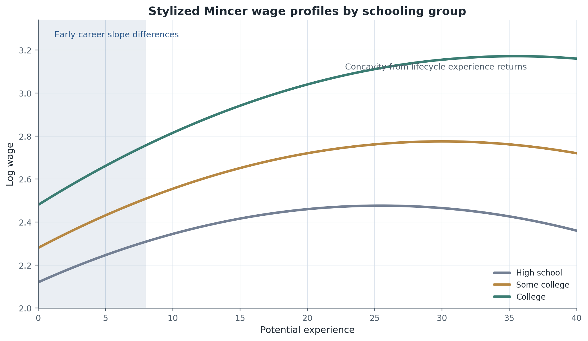
Figure 1:Stylized Mincer wage profiles by schooling group. The figure makes three teaching points at once: higher schooling can shift wage levels, alter experience slopes, and change the timing of concavity. That is why “the return to schooling” is not only a single intercept shift in practice.
Figure Figure 1 is a useful first lecture picture because it shows why Mincer-style estimates remain central even when they are incomplete. They summarize wage differences over the life cycle, discipline calibration, and provide the natural baseline against which causal and structural approaches are compared.
Field Core
Selection, comparative advantage, and heterogeneous gains
The first reason not to overread Equation (1) is that workers choose schooling, occupations, and locations. In a compact potential-outcomes representation,
where is the wage outcome person would obtain at schooling level , captures baseline productivity or market position, and allows the gain from schooling to vary across people. Equation (2) is deliberately minimal, but it forces the right question: if returns vary across individuals, who selects into more schooling?
The Roy and Willis-Rosen logic is stronger than a simple omitted-variable story. Selection is not only “high-ability people have more schooling.” It is also sorting on gains. Students choose schooling partly because the relative payoff to schooling differs across them, and those payoff differences can be linked to occupations, local labor markets, or access to firms Roy, 1951Willis & Rosen, 1979. That is why the OLS coefficient in Equation (1) blends prices, quantities, and endogenous selection.
This is also the point where Week 4 matters. If earlier investments changed both skill levels and the return schedule , then wage premia reflect cumulative advantage rather than one contemporaneous treatment. A field-course reading of returns-to-schooling evidence therefore has to distinguish three objects:
the descriptive gap in observed wages;
the causal effect of extra schooling for a specified margin;
the equilibrium pathway through which schooling changes access to occupations, firms, or places.
What does IV estimate?
Compulsory-schooling laws and related institutional rules were important because they forced returns-to-education research to specify which causal object an instrument identifies Card, 1999Oreopoulos, 2006. A compact local-return expression is
Equation (3) is the Week 5 discipline in one line. IV is not merely “OLS with a better source of variation.” It is a different estimand. The instrument identifies a local return for individuals whose schooling changes because the policy changes. Policy relevance depends on whether those compliers resemble the margin a policymaker cares about Oreopoulos, 2006Carneiro et al., 2011.
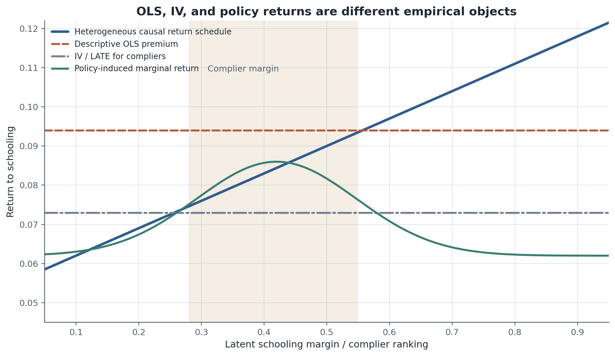
Figure 2:Conceptual comparison of descriptive OLS, IV/LATE, and policy-induced marginal returns. The point is not that one line is always above another. The point is that different designs recover different objects because they move different schooling margins.
Figure Figure 2 is helpful because it makes a point students often miss: changing the design changes the parameter, not only the standard error. Oreopoulos is valuable in class because compulsory-schooling laws “really matter” there; the first stage is economically meaningful, so the local-return interpretation is not cosmetic Oreopoulos, 2006. Stephens and Yang are equally valuable because they show that even a familiar instrument can be fragile if cohort trends or law coding are not handled carefully Stephens & Yang, 2014. Design credibility and target-parameter credibility are complements, not substitutes.
Table 1:Parameter map for returns-to-schooling research
| Object | Typical empirical design | What it measures | Main interpretive threat |
|---|---|---|---|
| Descriptive schooling premium | OLS Mincer regression | Conditional association between schooling and wages | Selection on ability, preferences, family background, and sorting |
| Average treatment effect (ATE) | Strong structural assumptions or experimental analogues | Mean causal gain from additional schooling for the target population | External validity and treatment heterogeneity |
| Local average treatment effect (LATE) | IV using compulsory-schooling or eligibility variation | Causal return for compliers at the policy margin shifted by the instrument | Margin-specific interpretation; compliers may differ across instruments |
| Marginal policy effect / MTE-style object | Structural or local instrumental-variables approaches | Return for individuals induced by a specific marginal policy change | Stronger functional-form and support requirements |
| Firm-mediated schooling return | Matched employer--employee decompositions or access-to-firm designs | Share of education premium operating through access to higher-paying firms | Firm effects may also bundle rents, amenities, and selection |
Table Table 1 is the cleanest way to keep the objects straight. OLS, ATE, LATE, marginal policy effects, and firm-mediated returns are not nested rhetorical refinements. They are distinct targets with distinct policy meanings.
Wages are also shaped by jobs, firms, and places
If Week 5 stopped with OLS versus IV, it would still be too narrow. Wages are set inside labor markets with heterogeneous firms and heterogeneous places. A compact worker-firm decomposition is
where is a worker effect, is the premium associated with firm , and captures observables such as experience. Equation (4) does not say that firm effects are pure rents or pure productivity; it says that observed wage dispersion can be decomposed into worker and firm components rather than being loaded entirely onto worker skill Abowd et al., 1999Card et al., 2018.
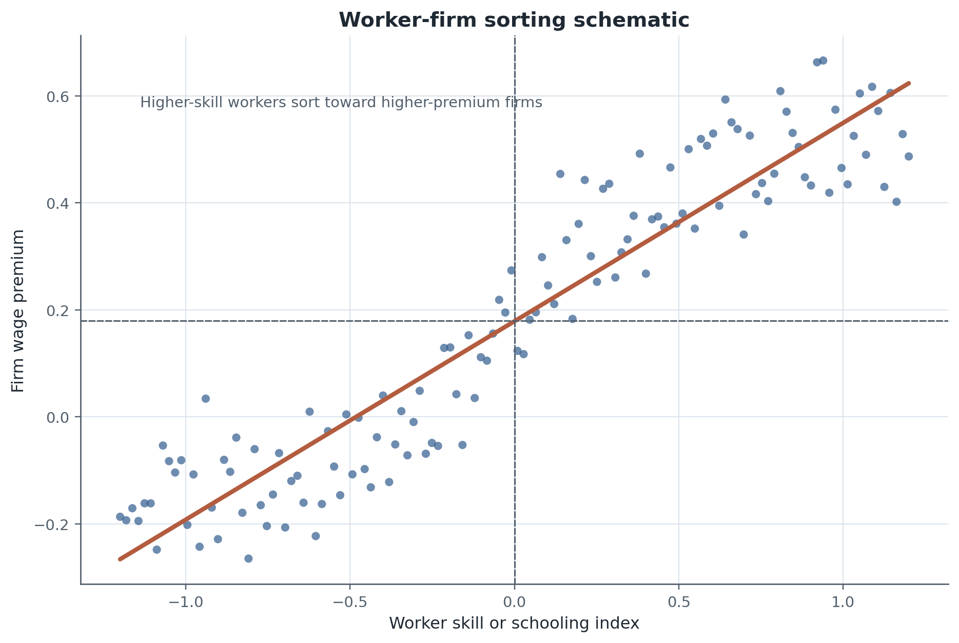
Figure 3:Worker-firm sorting schematic. Education and other skill measures can raise wages partly by shifting workers toward firms with higher wage premia rather than only by raising pay within a fixed firm.
Figure Figure 3 makes the firm-mediated channel visible. Engbom and Moser emphasize precisely this point for returns to education: part of the payoff to schooling can operate through access to higher-paying firms Engbom & Moser, 2017. Diamond makes the analogous point for places: some returns to skill are mediated by sorting into cities with steeper skill premia, different rents, and different amenity bundles Diamond, 2016.
Table 2:Conceptual sources of wage dispersion
| Source of wage differences | Core mechanism | Typical empirical approach | Why it matters for Week 5 |
|---|---|---|---|
| Worker skill and experience | Human capital and accumulated productive capacity | Wage equations, lifecycle profiles, structural accumulation models | Baseline interpretation of Mincer-style regressions |
| Selection and comparative advantage | Endogenous sorting into schooling, occupations, or sectors | Roy models, IV designs, control-function and structural selection models | Explains why descriptive premia need not equal causal returns |
| Firm wage premia | Heterogeneous pay policies, rents, bargaining, or efficiency wages | Matched employer--employee data, AKM decompositions | Education may pay partly by improving access to better firms |
| Compensating differentials | Nonwage amenities and job disamenities | Hedonic wage logic, job-attribute linked data | Wage gaps need not map directly into welfare or productivity |
| Location effects | Spatial wage premia, rents, amenities, and migration sorting | City or regional wage decompositions, spatial equilibrium designs | Some returns to skill are mediated by where workers sort |
Table Table 2 is the right transition from individual wage equations to broader inequality work. It separates productive skill, selection, firm premia, compensating differentials, and location effects. That separation is exactly what Week 8 inequality needs, because rising wage dispersion cannot be interpreted without knowing whether the movement came from skill prices, worker composition, firm dispersion, or sorting across markets Juhn et al., 1993Katz & Autor, 1999.
What empirical designs identify in wage-determination research
Week 5 evidence is easiest to organize by design bucket rather than by paper chronology.
Descriptive wage equations use cross-sectional or panel variation in schooling and experience to summarize conditional wage premia. They are useful for measurement, calibration, and lifecycle mapping, but the main threat is endogenous selection into schooling, occupations, and places.
Compulsory-schooling or law-based IV designs use institutional variation in minimum schooling requirements or eligibility rules. They target local returns for the margin shifted by the law, and the main threat is that the instrument may be entangled with cohort trends, law coding, or other contemporaneous changes.
Fixed-effects matched employer-employee decompositions use worker mobility across firms to separate worker and firm components. They are powerful for mapping wage dispersion, but interpretation remains contested because firm effects may bundle productivity, rents, bargaining, and amenities.
Spatial or firm-sorting designs use variation across cities, regions, or employer access. They show that schooling can pay through market assignment, but the main threat is endogenous mobility into places or firms whose premiums are themselves equilibrium objects.
Structural selection models use explicit assumptions on potential outcomes, costs, or marginal treatment effects. They can target policy-relevant counterfactuals, but they trade broader scope for stronger functional-form and support assumptions Heckman et al., 2006Carneiro et al., 2011.
Why Week 5 is the bridge week
Week 5 is where Labor I stops treating wages as simple reduced-form outcomes. Week 6 will show that household formation, care constraints, marriage, and fertility change both schooling choices and observed wages because the relevant decision-maker is often a household rather than an isolated worker. Week 7 will add compensating differentials and job amenities, making it even clearer that wages are incomplete welfare objects. Week 8 will take the final step and ask how dispersion evolves across workers, firms, and markets. The conceptual discipline built here is therefore cumulative: separate the parameter, the design, and the equilibrium pathway before drawing distributional conclusions.
Research Lab
The frontier challenge is not whether schooling matters, but which return object matters for the question at hand and through which market margin that return is realized. Modern wage-determination research sits at the intersection of human capital, selection, institutions, and market assignment. That is why Week 5 has to speak both to the classical returns-to-schooling literature and to modern worker-firm and worker-place decompositions Oreopoulos, 2006Card et al., 2018Engbom & Moser, 2017.
The bounded Week 5 lab reflects that agenda in a teachable way. Students reproduce an Oreopoulos-style compulsory-schooling comparison on a deterministic synthetic dataset, diagnose why the OLS and IV estimates target different objects, and then transfer the workflow to a Stephens and Yang-style trend-sensitivity exercise. An optional reflection note asks how a measured schooling return might partly operate through access to better firms or cities in the spirit of Engbom & Moser, 2017 or Diamond, 2016.
The chapter should also leave students with open research questions:
When does an observed schooling premium mostly reflect sorting rather than human-capital accumulation?
How stable are IV returns across different compulsory-schooling margins or cohorts?
How much of the return to education operates through access to better firms rather than through within-firm pay?
When do wage premia reflect amenities or rents instead of productivity differences?
Which return object should policy makers care about when evaluating a schooling subsidy or completion reform?
Methods Box
Week 5 adds one discipline to the Week 4 toolkit: never interpret a wage coefficient before naming the estimand and the market margin.
Start with Equation (1) as a benchmark accounting device, not as the final causal model.
Use Equation (2) to ask whether returns vary across people and whether selection is on levels, on gains, or both.
Use Equation (3) to state clearly when IV identifies a local policy-margin return rather than a universal effect.
Use Equation (4) to ask whether wage differences operate partly through firms or places instead of only within a worker-level return schedule.
Before using wage gaps for welfare or inequality claims, separate productivity, amenities, rents, and assignment effects.
Reading Ladder And References
Bridge
Roy on earnings distributions and selection Roy, 1951
Mincer on schooling, experience, and earnings profiles Mincer, 1974
Card’s guide to causal returns to education Card, 1999
Field Core
Willis and Rosen on education and self-selection Willis & Rosen, 1979
Heckman, Lochner, and Todd on earnings functions, treatment effects, and the limits of the Mincer equation Heckman et al., 2006
Oreopoulos on compulsory-schooling IV when the first stage is economically meaningful Oreopoulos, 2006
Stephens and Yang on trend sensitivity in compulsory-schooling designs Stephens & Yang, 2014
Carneiro, Heckman, and Vytlacil on marginal returns and local policy objects Carneiro et al., 2011
Research Lab
Abowd, Kramarz, and Margolis on worker and firm components of wages Abowd et al., 1999
Card, Cardoso, Heining, and Kline on firms and labor-market inequality Card et al., 2018
Engbom and Moser on returns to education through access to higher-paying firms Engbom & Moser, 2017
Diamond on diverging location choices by skill Diamond, 2016
Juhn, Murphy, and Pierce and Katz and Autor for the bridge to rising wage inequality Juhn et al., 1993Katz & Autor, 1999
Exercises And Discussion Prompts
Equation (1) treats the schooling premium as one coefficient. Use Figure Figure 1 to explain why lifecycle slope differences can still matter for interpretation even when the reported coefficient is a single average.
In Equation (2), what exactly distinguishes selection on levels from selection on gains, and why does the distinction matter for OLS interpretation?
Explain in words what Equation (3) identifies and why two valid instruments need not recover the same return.
Use Table Table 1 to compare a descriptive OLS premium, a LATE, and a marginal policy effect. Which of the three is closest to the object a policymaker wants when expanding compulsory schooling?
Figure Figure 3 shows positive worker-firm sorting. Give two reasons this can make the education premium larger even if within-firm pay schedules stay unchanged.
Why is Table Table 2 a necessary prelude to Week 8 inequality?
How might the household models from Week 6 change the interpretation of an estimated return to schooling for women or secondary earners?
Reproducibility And Code Lab Note
The Week 5 lab is organized around a bounded Reproduce -> Diagnose -> Transfer -> Reflect path that runs fully locally. Students reproduce one synthetic compulsory-schooling design in the spirit of Oreopoulos, 2006, diagnose why the resulting OLS and IV estimates are different empirical objects, and then transfer the workflow to a trend-sensitivity exercise in the spirit of Stephens & Yang, 2014. The smoke path avoids restricted matched employer-employee data and keeps the sorting extension optional and conceptual. The bounded workflow is documented in lab.md.
Slide Companion Note
The Week 5 deck should isolate the pricing problem rather than reproduce the chapter. It should move from the Week 4 human-capital bridge to the Mincer benchmark, selection and heterogeneous gains, OLS versus IV/LATE interpretation, worker-firm or worker-place sorting, the parameter map table, and the bridges to Week 6 households and Week 8 inequality. The canonical source is 05
Bridge Forward
Use this closing bridge to carry the module’s labor object, mechanism, and evidence into the next course step or research-design exercise.
- Mincer, J. (1974). Schooling, Experience, and Earnings. Columbia University Press.
- Card, D. (1999). The Causal Effect of Education on Earnings. In O. Ashenfelter & D. Card (Eds.), Handbook of Labor Economics (Vol. 3A, pp. 1801–1863). Elsevier. 10.1016/S1573-4463(99)03011-4
- Heckman, J. J., Lochner, L. J., & Todd, P. E. (2006). Earnings Functions, Rates of Return and Treatment Effects: The Mincer Equation and Beyond. In E. A. Hanushek & F. Welch (Eds.), Handbook of the Economics of Education (Vol. 1, pp. 307–458). Elsevier. 10.1016/S1574-0692(06)01007-5
- Roy, A. D. (1951). Some Thoughts on the Distribution of Earnings. Oxford Economic Papers, 3(2), 135–146. 10.1093/oxfordjournals.oep.a041827
- Willis, R. J., & Rosen, S. (1979). Education and Self-Selection. Journal of Political Economy, 87(5, Part 2), S7–S36.
- Card, D., Cardoso, A. R., Heining, J., & Kline, P. (2018). Firms and Labor Market Inequality: Evidence and Some Theory. Journal of Labor Economics, 36(S1), S13–S70. 10.1086/694153
- Diamond, R. (2016). The Determinants and Welfare Implications of US Workers’ Diverging Location Choices by Skill: 1980–2000. American Economic Review, 106(3), 479–524. 10.1257/aer.20131706
- Abowd, J. M., Kramarz, F., & Margolis, D. N. (1999). High Wage Workers and High Wage Firms. Econometrica, 67(2), 251–333. 10.1111/1468-0262.00020
- Oreopoulos, P. (2006). Estimating Average and Local Average Treatment Effects of Education when Compulsory Schooling Laws Really Matter. American Economic Review, 96(1), 152–175. 10.1257/000282806776157641
- Carneiro, P., Heckman, J. J., & Vytlacil, E. (2011). Estimating Marginal Returns to Education. American Economic Review, 101(6), 2754–2781. 10.1257/aer.101.6.2754
- Stephens, Jr., Melvin, & Yang, D.-Y. (2014). Compulsory Education and the Benefits of Schooling. American Economic Review, 104(6), 1777–1792. 10.1257/aer.104.6.1777
- Engbom, N., & Moser, C. (2017). Returns to Education through Access to Higher-Paying Firms: Evidence from US Matched Employer-Employee Data. American Economic Review: Papers and Proceedings, 107(5), 374–378. 10.1257/aer.p20171013
- Juhn, C., Murphy, K. M., & Pierce, B. (1993). Wage Inequality and the Rise in Returns to Skill. Journal of Political Economy, 101(3), 410–442. 10.1086/261881
- Katz, L. F., & Autor, D. H. (1999). Changes in the Wage Structure and Earnings Inequality. In O. Ashenfelter & D. Card (Eds.), Handbook of Labor Economics (Vol. 3A, pp. 1463–1555). Elsevier.