Inequality and Wage Dispersion
Learning Objectives
By the end of Week 8, students should be able to:
distinguish hourly wage inequality, annual earnings inequality, hours and employment inequality, total job-value inequality, and household inequality;
define quantile-based and variance-based inequality objects and explain why they answer different empirical questions;
write down and interpret a between-group versus within-group variance decomposition;
explain what residual inequality means in a descriptive wage equation and why it became central after Juhn et al., 1993;
connect the college premium, task polarization, institutions, firm premia, and sorting to different parts of the wage distribution rather than to one master mechanism;
interpret linked employer-employee decompositions in the spirit of Card et al., 2018 and Song et al., 2019;
explain why Week 7’s amenity logic implies that wage inequality and total labor-market value inequality are not the same object;
see why Week 9 discrimination and segmentation require this distributional architecture rather than replacing it.
Opening Orientation
The economic question for the week is deliberately broader than in earlier modules: once Weeks 5 and 6 have explained how wages and households convert market opportunities into realized outcomes, and Week 7 has shown that wages do not exhaust job value, how should labor economists measure inequality and organize the mechanisms that shape the distribution of labor-market outcomes Autor et al., 2008Card et al., 2018Song et al., 2019?
Bridge
Week 5 put wage determination at the center of the worker side of labor economics. Week 6 showed that households transform wages into hours, participation, and realized earnings. Week 7 added the crucial correction that jobs are bundles of wages plus amenities, so measured pay is not the whole labor-market opportunity set. Week 8 now asks how those objects aggregate into inequality.
That move matters because inequality is not one number attached to one outcome. Hourly wages, annual earnings, hours, employment, total compensation, and household resources can all tell different stories. A rise in annual-earnings inequality may come from wider hourly wage dispersion, weaker hours for the lower tail, more nonemployment, or all three. A rise in wage inequality may overstate or understate welfare inequality if desirable amenities sort with high-pay jobs. Before students ask why inequality changed, they need to know which distribution they are studying and which margin is actually moving Lemieux, 2006Autor et al., 2008.
Field Core
Inequality is not one object
The first discipline is to separate the empirical object from the explanation. The weekly source pack insists on this because many disagreements in the inequality literature are really disagreements about what is being measured. For wage-setting questions, hourly wages are often the cleanest object because they strip out many hours and employment margins. For labor-market well-being, annual earnings are often more relevant because they incorporate the quantity of work supplied. For welfare-oriented questions, even annual earnings can be too narrow because Week 7 showed that workers care about schedule control, safety, stability, commute burden, and autonomy as part of compensation.
Table 1:Inequality concepts map
| Empirical object | What it captures | What it misses | When it is the right object |
|---|---|---|---|
| Hourly wages | Price of labor per hour worked; cleanest object for wage-setting questions | Hours, employment, nonwage amenities, household insurance | Skill prices, returns to schooling, firm premia |
| Annual earnings | Combined effect of wages, hours, weeks, and employment margins | Nonwage job quality; household sharing | Labor-market well-being when nonemployment/hours are central |
| Hours / employment | Quantity margins and participation inequality | Wage-setting unless combined with pay data | Household allocation, extensive-margin policy, labor-force attachment |
| Total compensation / job value | Wages plus amenity value, schedule quality, safety, flexibility, and stability | Hard to observe directly; requires valuation assumptions | Welfare-oriented comparisons across jobs or groups |
| Household income | Post-labor pooling, transfers, and family insurance | Individual labor-market mechanisms can be obscured | Broader living-standards or family-incidence analysis |
Table Table 1 should anchor the opening discussion. The field-course point is not that one object is universally best. It is that different objects answer different questions. That is why the same economy can exhibit moderate hourly wage dispersion, much larger annual earnings dispersion, and an even different ranking once total job value is monetized.
Measurement architecture: distributions, percentiles, and interpretation
Let denote the wage distribution in period , and let denote its -quantile. The most teachable compact object for this week is
Equation (1) makes two ideas visible. First, inequality comparisons are comparisons of functions of distributions, not only of means. Second, upper-tail and lower-tail movements can be separated. The statistics and isolate the upper and lower halves of the wage distribution; a change in one need not imply the same change in the other Autor et al., 2008.
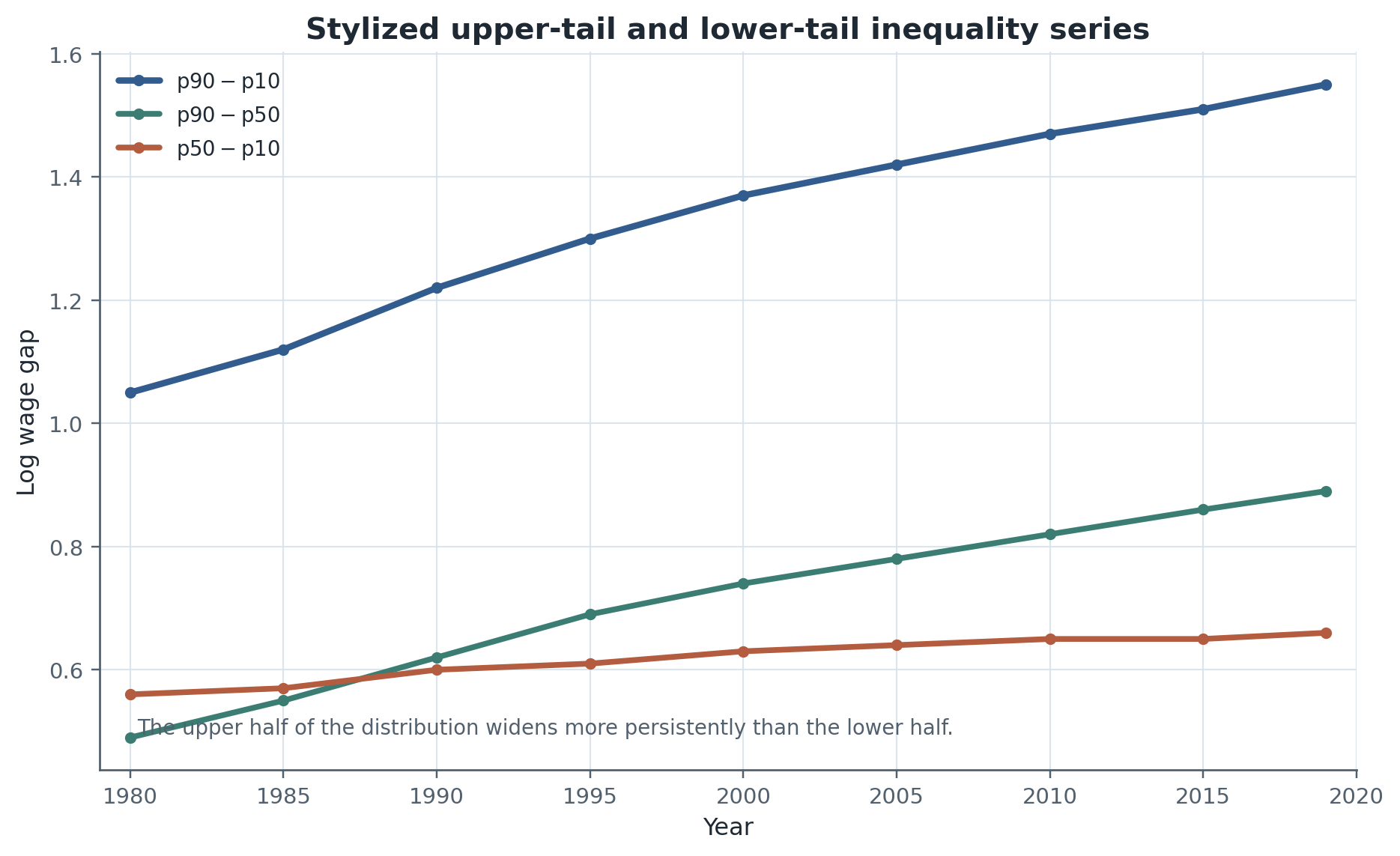
Figure 1:Stylized percentile-gap series for log wages. The figure emphasizes that upper-tail and lower-tail inequality need not move together, even when the full spread rises.
Figure Figure 1 is the cleanest way to explain why quantile objects became canonical. If rises while is flat or falling, then a model aimed at the entire distribution is already too coarse. That is one reason the post-1980 literature split upper-tail inequality, lower-tail inequality, and middle compression into separate but related facts Juhn et al., 1993Autor et al., 2008.
Variance-based measures play a different role. The log variance compresses the entire distribution into one scalar and is especially convenient for decomposition. But it weights the tails differently from percentile gaps and can react strongly to top-end changes. Top shares add yet another lens, especially when the upper tail becomes sufficiently influential that broad quantile summaries hide what is happening above the or . A serious chapter therefore teaches percentile gaps, log-variance measures, and the conceptual role of top shares without pretending they are interchangeable.
The measurement lesson from Week 7 belongs here too. If desirable amenities are concentrated among high-wage jobs, wage inequality understates inequality in total labor-market value. If workers accept lower wages for flexibility or safety, wage inequality can overstate welfare inequality. Measurement is therefore not separate from welfare interpretation; it disciplines it.
Between-group, within-group, and residual inequality
Once the object is defined, the next question is where dispersion sits. A basic decomposition groups workers by education, occupation, place, industry, or firm and asks how much wage dispersion comes from gaps between group means versus inequality within groups. The compact variance accounting identity is
Equation (2) is descriptive, but it is not trivial. If inequality rises because group means diverge, then compositional or price changes across observed categories are important. If inequality rises mostly within groups, then the field needs richer heterogeneity, unobservables, institutions, or firm-level margins to explain the data Juhn et al., 1993Lemieux, 2006.
The wage-equation version of the same idea is
where might include education, experience, gender, occupation, region, or other observables. Equation (3) does not claim that the residual is a structural primitive. It says only that some part of inequality remains after conditioning on measured characteristics. The empirical surprise documented in the classic literature is that residual inequality increased substantially even when observable composition shifts alone were not large enough to explain the full rise Juhn et al., 1993Lemieux, 2006.
Students should be taught to read the residual carefully. It is not “pure skill.” It mixes unobserved productivity, rent sharing, measurement error, bargaining, job ladders, task differences, and omitted institutions. But the residual is still informative because it tells the field where simple observables stop being enough.
Canonical facts: what changed and where in the distribution
The durable facts are easier to teach than the chronology of papers.
First, upper-tail wage inequality rose strongly after 1980. Second, lower-tail dynamics were more time-specific: institutional changes and macro conditions matter more for the lower half of the distribution than a single smooth long-run trend would suggest Autor et al., 2008. Third, the college premium increased, but it did not fully summarize all relevant inequality changes. Fourth, occupational and task patterns look polarized rather than uniformly skill-upgraded in many subperiods, especially once middle routine work is separated from both low-wage service work and high-skill abstract work Autor & Dorn, 2013Acemoglu & Autor, 2011.
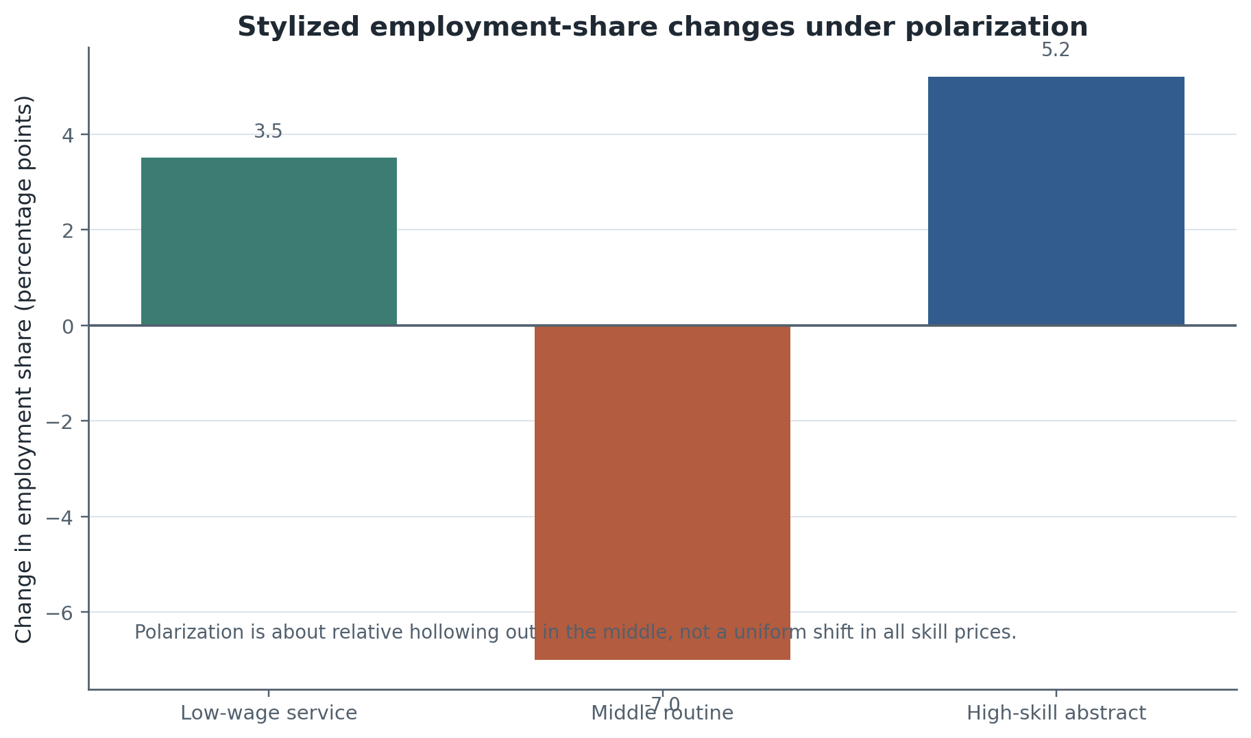
Figure 2:Stylized employment-share changes under polarization. The point is not the exact magnitudes but the pattern: relative decline in middle routine work together with stronger low- and high-end growth.
Figure Figure 2 is useful because it keeps polarization distinct from a one-dimensional skill-premium story. A rising college premium and a hollowing out of middle routine work can be related, but they are not identical facts. This is why the mechanism discussion has to separate broad supply-demand logic from task reallocation and lower-tail institutions Katz & Murphy, 1992Autor & Dorn, 2013.
Composition also matters. If the workforce becomes more educated, older, more female, more urban, or more concentrated in particular sectors, raw inequality changes may mix prices and quantities. The great contribution of reweighting and decomposition work was to show how composition-adjusted distributions can tell a cleaner story about changes in returns, institutions, and residual dispersion DiNardo et al., 1996Firpo et al., 2009.
Mechanism block I: supply, demand, tasks, and technology
The cleanest starting point is still Katz-Murphy style supply-demand logic. If relative demand for skill rises faster than relative supply, the skill premium increases Katz & Murphy, 1992Katz & Autor, 1999. That logic remains foundational because it ties Week 8 back to Week 4 human capital and Week 5 returns to skill. Workers differ in accumulated skill, firms demand bundles of tasks, and equilibrium prices adjust.
But that framework is not the end of the story. The task-based literature makes clear that technology can substitute more directly for routine middle tasks while complementing abstract tasks and leaving many low-wage service tasks less exposed to direct automation. This generates a pattern that looks less like a smooth rise in one latent skill price and more like distributional reshaping across occupations and tasks Acemoglu & Autor, 2011Autor & Dorn, 2013.
The right classroom discipline is to ask what each mechanism explains well. Supply-demand logic is strong on long-run skill premiums. Task-based logic is strong on middle compression and occupational reallocation. Neither one by itself explains every lower-tail movement, every firm pattern, or every place-based divergence.
Mechanism block II: institutions and the lower tail
Lower-tail and middle-distribution movements are hard to read without institutions. Minimum wages, unions, bargaining norms, and wage-setting rules compress or decompress specific parts of the distribution rather than shifting all percentiles equally. This is one reason the lower tail is often more episodic and policy-sensitive than the persistent upper-tail rise DiNardo et al., 1996Autor et al., 2008.
DiNardo, Fortin, and Lemieux provide the conceptual bridge here. Their counterfactual reweighting logic asks how the wage distribution would have looked under alternative compositions or institutional environments without requiring the researcher to pretend that one reduced-form coefficient summarizes the entire distribution DiNardo et al., 1996. The field-course lesson is not just a method lesson. It is substantive: institutional explanations are often segment-specific. A fall in union coverage or a change in the minimum wage can matter a lot for while saying far less about the top tail.
That is why Week 8 should resist global narratives. Institutions can be central for the lower tail and still be incomplete as an explanation for upper-tail growth. Conversely, a technology-based account may fit upper-tail or middle reallocation facts and still leave the lower tail underexplained.
Mechanism block III: firms, rents, sorting, and geography
The modern frontier added a new level of analysis: the employer. In linked employer-employee data, one can write
where is a worker effect, is the wage premium paid by the worker’s firm, and captures observables. Equation (4) is not the whole truth about wage setting, but it sharply organizes the question. How much inequality reflects persistent worker heterogeneity, how much reflects wage-setting differences across firms, and how much reflects positive sorting between high-wage workers and high-premium firms Card et al., 2018Song et al., 2019?
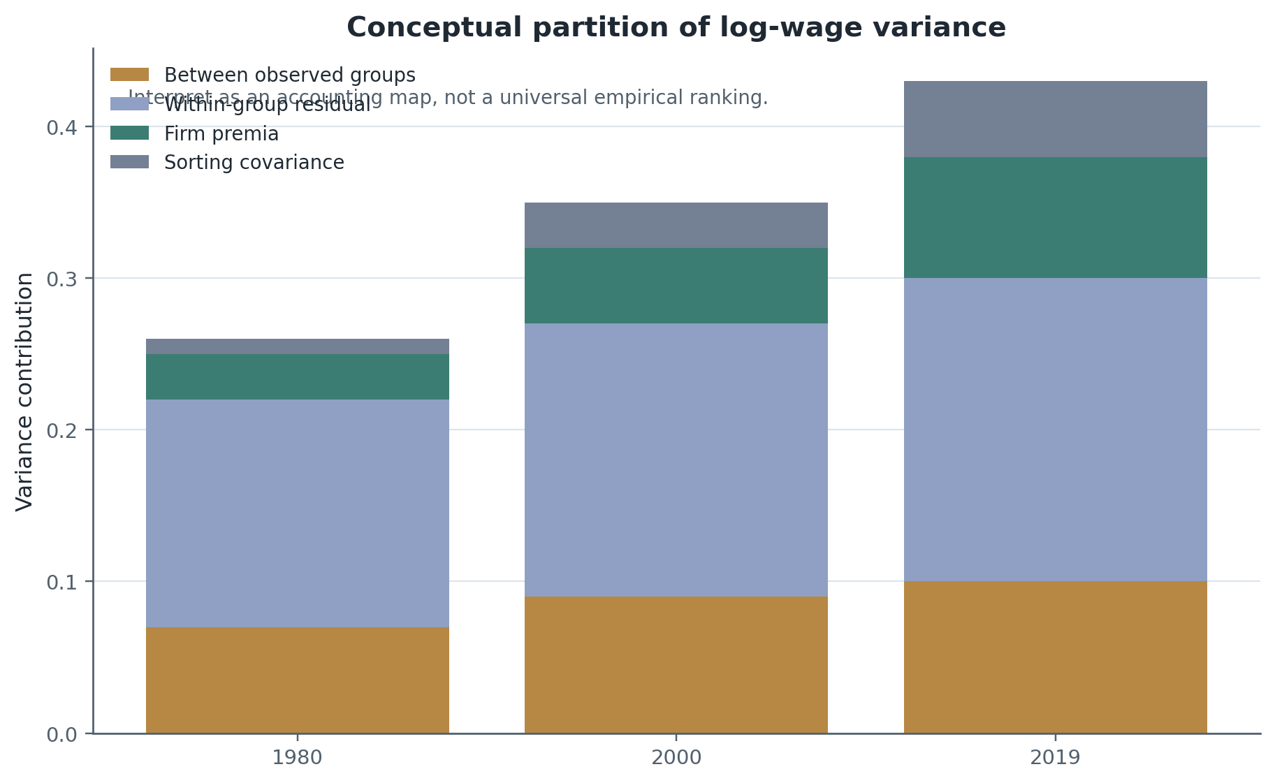
Figure 3:Conceptual stacked decomposition of wage-dispersion components. It visualizes the accounting distinction among between-group terms, within-group residual inequality, firm premia, and worker-firm sorting.
Figure Figure 3 helps because students can otherwise treat firm inequality as a separate topic rather than as a decomposition of worker outcomes. The firm block changed the field because it showed that between-firm pay dispersion and worker-firm sorting can account for a meaningful share of wage inequality. It also opened the door to place-based interpretations, since local labor markets differ in industry mix, firm composition, outside options, and rent-sharing environments Card et al., 2018Song et al., 2019.
Geography enters naturally here. If high-premium firms cluster spatially, wage inequality becomes partly an allocation problem across places as well as across firms. This is not yet Week 10 mobility, but it is the bridge to it. Where workers live and which firms they can reach become part of the architecture of inequality.
Welfare, total labor-market value, and the bridge from Week 7
Week 7’s most important gift to Week 8 is skepticism about wages as a sufficient welfare statistic. A compact bridge object is
where is wages and is the monetized value of amenities, schedule quality, stability, safety, or other nonwage job attributes. Equation (5) is deliberately spare. Its job is to stop students from unconsciously equating wage dispersion with inequality in labor-market opportunity sets.
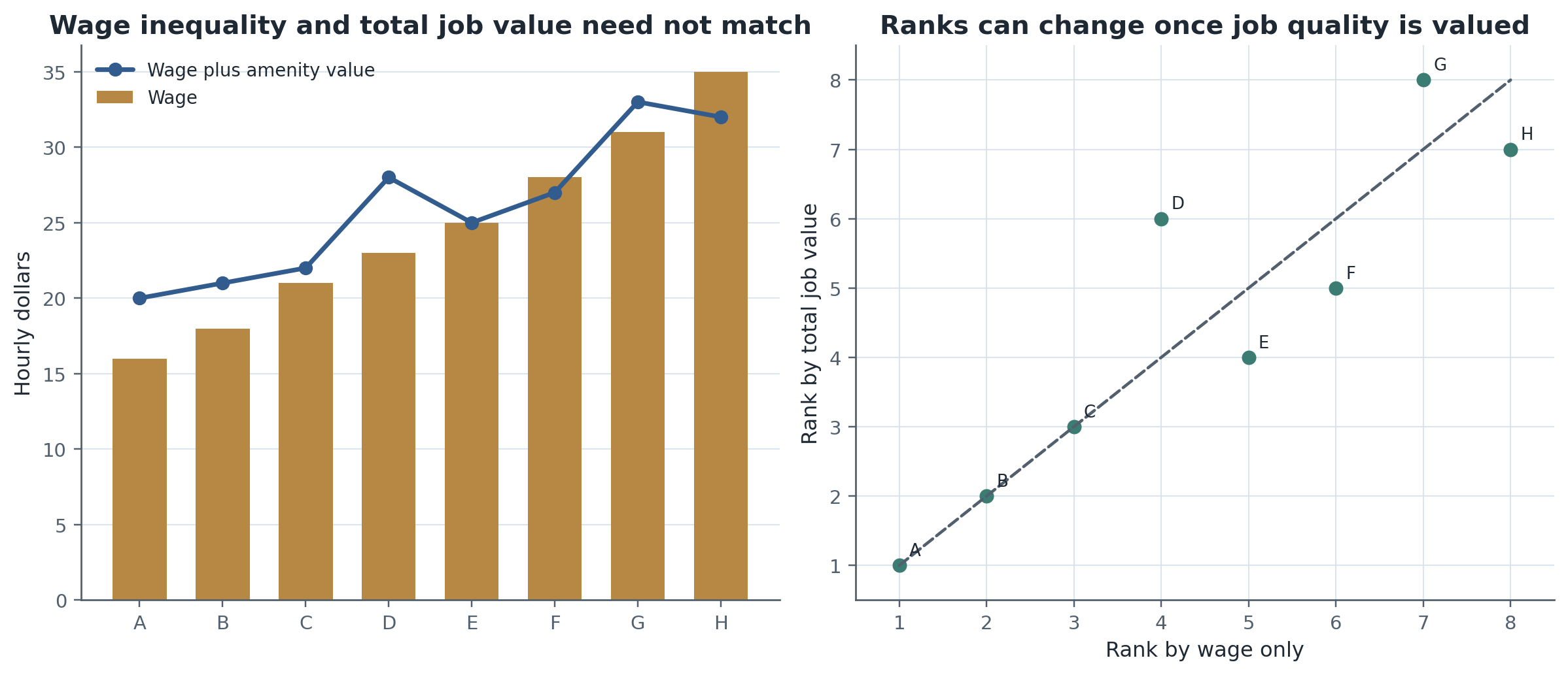
Figure 4:Conceptual comparison of wage-only and total job-value rankings. Accounting for amenities can flatten, steepen, or reorder measured inequality depending on how nonwage job quality sorts across workers and firms.
Figure Figure 4 shows why the bridge matters. If high-wage firms also offer safer conditions, more stable schedules, and lower risk, then inequality in total job value exceeds wage inequality. If some workers accept lower wages for flexibility or location, then wage inequality may overstate welfare inequality. Empirically, Week 8 still centers wages and earnings because those are far better observed than full job value. Conceptually, however, the Week 7 correction must remain in view Card et al., 2018.
Research Lab
The bounded Week 8 lab is built around a local Reproduce -> Diagnose -> Transfer workflow that does not require restricted administrative data. The reproduction step uses a synthetic CPS-style file to recover a small inequality factbook in the spirit of Autor et al., 2008: percentile gaps, a college premium comparison, a between-versus-within decomposition, and a residual-inequality summary. This keeps the core inequality objects transparent and reproducible.
The diagnostic step asks students to separate descriptive decomposition from causal explanation. A rising residual component in Equation (3) is not a stand-alone mechanism. Students must say what the residual may bundle together and which facts it helps discipline. The transfer step then moves to a synthetic linked employer-employee panel that supports a simple worker-firm decomposition in the spirit of Card et al., 2018 and Song et al., 2019. The aim is not to mimic confidential-data scale. It is to teach the logic of worker effects, firm premia, and sorting.
An optional extension note points students toward Haanwinckel, 2025 for a broader synthesis of supply, firms, institutions, and the wage distribution. The bounded path stays deliberately local and pedagogical. It teaches the architecture of modern inequality analysis without pretending that a teaching dataset can replicate the entire administrative-data frontier.
Open research questions should remain visible:
Which parts of rising inequality are best understood as price changes versus allocation changes?
How robust are firm-premium decompositions to design choices, connected-set restrictions, and imperfect mobility?
When do amenities amplify wage inequality and when do they offset it?
Which inequality object is best for policy incidence when hours, employment, and household insurance move at the same time?
How should Week 9 discrimination work separate group-specific barriers from general dispersion in firms, tasks, and places?
Methods Box
Methods Box 1: distributional statistics and decomposition
Use Equation (1) when the question is where in the distribution change occurs. Use Equation (2) when the question is how much inequality lives between observed groups versus within them. Use Equation (3) when you need a compact descriptive accounting of what observables do and do not explain. The main discipline is to keep these objects descriptive unless the design truly identifies a causal counterfactual Juhn et al., 1993Firpo et al., 2009.
Methods Box 2: linked employer-employee inequality methods
Equation (4) is powerful because it makes firm heterogeneity explicit, but it needs panel mobility, a connected worker-firm graph, and careful interpretation. It is an accounting framework for worker effects, firm premia, and sorting. It is not automatically a model of bargaining, rents, monopsony, or welfare without further structure Card et al., 2018Song et al., 2019.
Table 2:Empirical toolkit map for inequality analysis
| Method | Main use | Data requirement | Main limitation |
|---|---|---|---|
| Percentile-series description | Track upper-tail, middle, and lower-tail changes over time | Repeated cross-sections or panels with consistent pay measures | Descriptive only; mechanism is not identified |
| Juhn--Murphy--Pierce style residual decomposition | Separate observed-characteristic changes from residual inequality | Rich micro data with stable covariates | Residual mixes many mechanisms and measurement issues |
| DiNardo--Fortin--Lemieux counterfactuals | Construct reweighted distributional counterfactuals for composition/institution changes | Repeated cross-sections with overlap | Requires support/overlap and remains partially descriptive |
| RIF / unconditional quantile methods | Estimate how covariates shift different points of the outcome distribution | Micro data and influence-function implementation | Interpretation depends on chosen functional and reweighting assumptions |
| AKM linked employer--employee decomposition | Partition wages into worker effects, firm premia, and sorting | Linked worker-firm panel data | Requires strong mobility/connected-set structure and can be sensitive to design choices |
Table Table 2 is the summary tool for the week. Each method answers a different inequality question, requires different data, and comes with a different limitation. Students should leave Week 8 knowing why papers that all study “inequality” can still be asking fundamentally different empirical questions.
Table 3:Mechanism map for labor-market inequality
| Mechanism | Distributional signature | Part of distribution most affected | Canonical evidence / logic |
|---|---|---|---|
| Skill supply and demand | Rising education or skill premiums when relative demand outpaces supply | Often upper half, but can affect the full distribution | Katz-Murphy style quantity-price logic |
| Tasks / polarization | Middle compression with relatively stronger low- and high-end growth or employment reallocation | Middle and upper-middle | Task-based and routine-biased technological change |
| Institutions | Compression or decompression at the lower tail and middle through bargaining power and wage floors | Lower tail and middle | Minimum wage, unions, and wage-setting institutions |
| Firms, rents, and sorting | Larger dispersion across employers and stronger matching between high-wage workers and high-premium firms | Can reshape the entire distribution | AKM decompositions, rent-sharing, and linked employer--employee data |
| Amenities / job quality | Wage gaps may understate or overstate welfare inequality depending on sorting in nonwage attributes | Any part of the distribution; often interacts with family constraints | Week 7 job-quality logic |
Table Table 3 is the parallel mechanism summary. It prevents the lecture from collapsing into either a one-mechanism story or an unstructured list of facts.
Reading Ladder And References
Bridge
Katz and Murphy on relative supply, relative demand, and wage structure Katz & Murphy, 1992
Juhn, Murphy, and Pierce on observed versus residual inequality Juhn et al., 1993
Autor, Katz, and Kearney for the field’s compact map of upper-tail, lower-tail, and polarization facts Autor et al., 2008
Field Core
Katz and Autor on the broader wage-structure synthesis Katz & Autor, 1999
DiNardo, Fortin, and Lemieux on composition and institutional counterfactuals DiNardo et al., 1996
Lemieux on composition, residual inequality, and interpretation Lemieux, 2006
Acemoglu and Autor on task-based technology and wage structure Acemoglu & Autor, 2011
Autor and Dorn on task polarization and middle compression Autor & Dorn, 2013
Firpo, Fortin, and Lemieux on distributional methods beyond means Firpo et al., 2009
Research Lab
Card, Cardoso, Heining, and Kline on worker-firm heterogeneity and sorting Card et al., 2018
Song, Price, Guvenen, Bloom, von Wachter on firming-up inequality through firms and rents Song et al., 2019
Haanwinckel as an optional frontier extension linking distributional mechanisms in a broader equilibrium frame Haanwinckel, 2025
Exercises And Discussion Prompts
Use Equation (1) to explain why a rise in does not imply the same change in .
In Table Table 1, which empirical object is best for a policy question about labor-force attachment, and which is best for a question about wage-setting? Why are they different?
Equation (2) is descriptive. Give one reason it is still highly informative for theory choice.
In Equation (3), why is it a mistake to interpret as a single structural force such as “technology”?
Compare the explanatory reach of Katz-Murphy style supply-demand logic and task-polarization logic. Which facts does each fit best?
Why can minimum wages or unions change more strongly than ?
Use Equation (4) to explain how firm premia and positive sorting can both raise wage inequality.
In Equation (5), under what sorting pattern would total labor-market value inequality exceed wage inequality?
Why does Week 8 have to come before Week 9 discrimination and segmentation if the class wants to interpret group gaps carefully?
Reproducibility And Code Lab Note
The Week 8 lab follows the standard bounded Reproduce -> Diagnose -> Transfer path. Students first build a synthetic inequality factbook in the spirit of Autor et al., 2008, then diagnose what percentile gaps, between-within decompositions, and residual inequality do and do not identify, and finally transfer the workflow to a synthetic worker-firm decomposition in the spirit of Card et al., 2018 and Song et al., 2019. The bounded workflow is documented in lab.md.
Slide Companion Note
The Week 8 deck should not reproduce the chapter verbatim. It should isolate the week’s architecture: why the module is heavier than usual, how Weeks 5--7 feed into distributional analysis, which inequality objects matter, how percentile gaps differ from variance decompositions, why the lower tail and upper tail need not share a mechanism, what linked employer-employee data changed, and why Week 9 discrimination must be read against this broader inequality map. The canonical source is 08
Bridge Forward
Use this closing bridge to carry the module’s labor object, mechanism, and evidence into the next course step or research-design exercise.
- Juhn, C., Murphy, K. M., & Pierce, B. (1993). Wage Inequality and the Rise in Returns to Skill. Journal of Political Economy, 101(3), 410–442. 10.1086/261881
- Card, D., Cardoso, A. R., Heining, J., & Kline, P. (2018). Firms and Labor Market Inequality: Evidence and Some Theory. Journal of Labor Economics, 36(S1), S13–S70. 10.1086/694153
- Song, J., Price, D. J., Guvenen, F., Bloom, N., & von Wachter, T. (2019). Firming Up Inequality. The Quarterly Journal of Economics, 134(1), 1–50. 10.1093/qje/qjy025
- Autor, D. H., Katz, L. F., & Kearney, M. S. (2008). Trends in U.S. Wage Inequality: Revising the Revisionists. The Review of Economics and Statistics, 90(2), 300–323. 10.1162/rest.90.2.300
- Lemieux, T. (2006). Increasing Residual Wage Inequality: Composition Effects, Noisy Data, or Rising Demand for Skill? American Economic Review, 96(3), 461–498. 10.1257/aer.96.3.461
- Haanwinckel, D. (2025). Supply, Demand, Institutions, and Firms: A Theory of Labor Market Sorting and the Wage Distribution. American Economic Review, 115(12), 4137–4182. 10.1257/aer.20201293
- Autor, D. H., & Dorn, D. (2013). The Growth of Low-Skill Service Jobs and the Polarization of the U.S. Labor Market. American Economic Review, 103(5), 1553–1597. 10.1257/aer.103.5.1553
- Acemoglu, D., & Autor, D. H. (2011). Skills, Tasks and Technologies: Implications for Employment and Earnings. In O. Ashenfelter & D. Card (Eds.), Handbook of Labor Economics (Vol. 4B, pp. 1043–1171). Elsevier. 10.1016/S0169-7218(11)02410-5
- Katz, L. F., & Murphy, K. M. (1992). Changes in Relative Wages, 1963–1987: Supply and Demand Factors. The Quarterly Journal of Economics, 107(1), 35–78. 10.2307/2118323
- DiNardo, J., Fortin, N. M., & Lemieux, T. (1996). Labor Market Institutions and the Distribution of Wages, 1973–1992: A Semiparametric Approach. Econometrica, 64(5), 1001–1044. 10.2307/2171954
- Firpo, S., Fortin, N. M., & Lemieux, T. (2009). Unconditional Quantile Regressions. Econometrica, 77(3), 953–973. 10.3982/ECTA6822
- Katz, L. F., & Autor, D. H. (1999). Changes in the Wage Structure and Earnings Inequality. In O. Ashenfelter & D. Card (Eds.), Handbook of Labor Economics (Vol. 3A, pp. 1463–1555). Elsevier.