Mobility, Migration, and Intergenerational Transmission
Learning Objectives
By the end of Week 10, students should be able to:
distinguish employer, occupation, place, and intergenerational mobility objects;
interpret transition matrices, hazard rates, rank-rank slopes, and wage-growth objects as distinct labor-market statistics;
explain how linked employer-employee data changed the study of worker mobility and firm sorting;
write down a migration-choice object with Roy-style selection and moving frictions;
explain what lottery, reform, border, and exposure designs identify in mobility and migration research;
distinguish descriptive persistence objects from causal transmission mechanisms in intergenerational mobility;
connect place, firm, and occupational mobility to inequality persistence rather than treating them as separate topics;
see why Week 11 worker-side policy is partly about relaxing mobility frictions rather than only changing static incentives.
Opening Orientation
The economic question for the week is dynamic but still labor-economic at its core. Once Week 9 has shown that workers may enter segmented opportunity sets, Week 10 asks how workers move across employers, occupations, and places, how much those moves raise wages or job quality, and why labor-market position still persists so strongly across families Jia et al., 2023Song et al., 2019Chetty et al., 2014.
Bridge
Week 9 ended with a deliberately uncomfortable point: the opportunity set through which workers search, move, and bargain may already be segmented by identity, firm behavior, and local opportunity. Week 10 keeps that insight but changes the question. Instead of asking whether treatment differs across workers at a point in time, we ask who moves, where they move, what those moves buy them, and why mobility is so uneven across firms, places, and generations.
This week matters because mobility has two opposing interpretations. In one interpretation, mobility is a margin of adjustment that reallocates labor toward better matches, higher-paying firms, and more productive places. In the other, mobility is precisely the margin that constraints suppress: moving is costly, information is incomplete, credit is limited, housing is scarce, and networks are unequal Diamond, 2016Kennan & Walker, 2011Van Doornik et al., 2024. A low mobility rate can therefore mean either stable good matches or trapped workers. The empirical task is to tell those stories apart.
Week 10 also bridges directly into Week 11. If workers do not move because credit, information, migration restrictions, or family background limit access to opportunity, then worker-side policy is not only about taxes and transfers. It is also about mobility margins: search assistance, moving support, migration access, training ladders, and place-sensitive policy design.
Field Core
Mobility objects after Week 9: transitions, hazards, and wage growth
The first discipline is not to say “mobility” as if it were one number. Let denote a worker’s employer-premium quartile, occupation tier, or place type at time , and let indicate a move between and . A transition-matrix object is
Equation (1) is descriptive but central. It tells us whether mobility is mostly lateral, upward, or downward. A hazard object,
asks which workers move, from which starting positions, and under which aggregate conditions. Neither object is causal by itself. Both are measurement devices that organize the dynamic allocation problem.
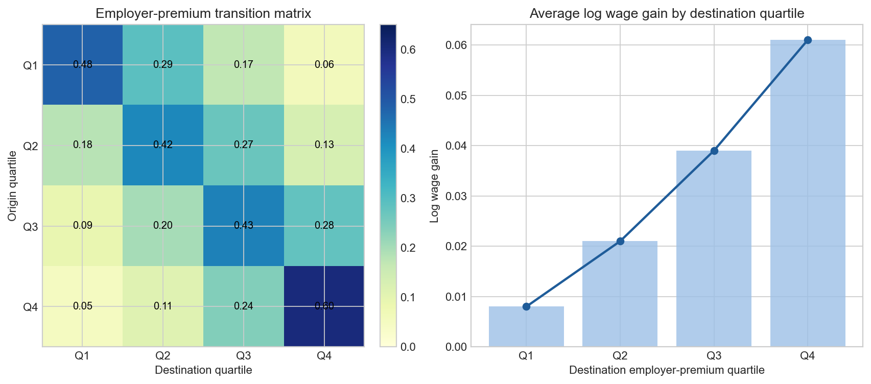
Figure 1:Transition matrices summarize where movers go, not just whether they move. The same employer-to-employer rate can hide very different patterns of upgrading, downgrading, and persistence across firm or occupation ladders.
The labor interpretation becomes sharper once wage growth is attached to the move. With linked employer-employee data, the field can study whether wage gains are tied to movement toward higher-premium firms, occupational upgrading, or better places rather than merely to generic turnover Abowd et al., 1999Card et al., 2013Engbom & Moser, 2017. A compact wage-growth object is
where is the firm wage premium. Equation (3) is useful because it keeps the lecture labor-focused. A move matters when it changes a worker’s position on a firm, occupation, or place ladder, not simply because the worker’s address changed.
Measurement improved substantially once researchers stopped relying only on household surveys to count employer-to-employer flows. Survey nonresponse, multiple-job ambiguity, and timing error can make job-to-job mobility look flatter and less cyclical than it really is. Measurement-correction work using richer linked records therefore changed a first-order labor fact, not a technical footnote Fujita et al., 2024.
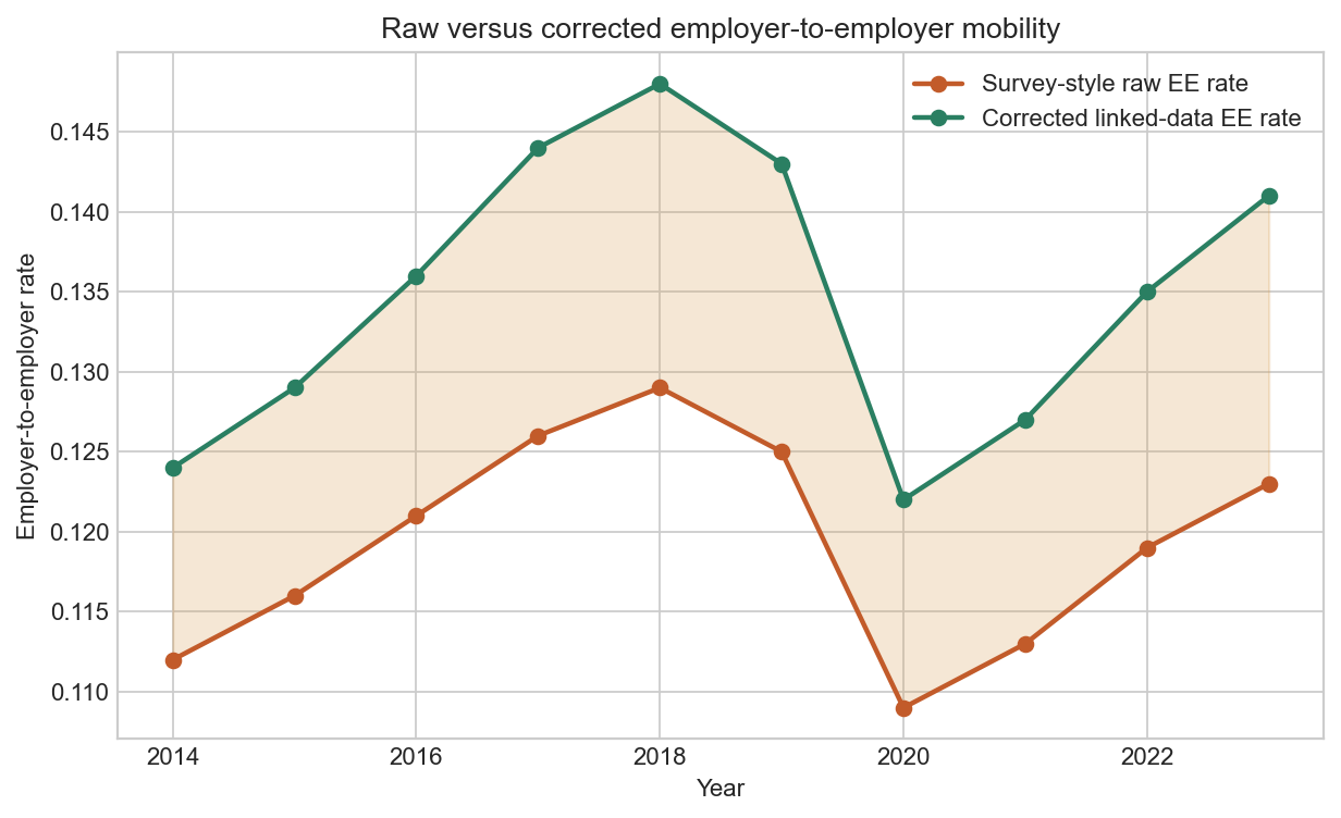
Figure 2:Correcting employer-to-employer mobility measurement can materially change the estimated level and cyclicality of reallocation. This is measurement progress, not a causal design.
Table 1:Mobility objects in labor economics
| Object | Typical empirical measure | Labor interpretation | Common identification or measurement issue |
|---|---|---|---|
| Employer-to-employer mobility | Employer-change indicator, EE flow rate, transition matrix | Reallocation across wage ladders and match qualities | Survey nonresponse, multiple-job ambiguity, timing of employer changes |
| Occupational mobility | Occupation transition matrix, upgrade/downgrade rate | Skill reallocation and task upgrading | Reclassification error, coarse occupation codes |
| Geographic migration | Move rate, distance moved, region transition, commuting expansion | Access to alternative local labor markets | Amenity confounding, housing constraints, selection into movers |
| Wage mobility | Earnings growth around employer, occupation, or place moves | Returns to movement across opportunity sets | Composition changes, anticipatory behavior |
| Intergenerational income mobility | Rank-rank slope, IGE, quintile transition matrix | Persistence of labor-market position across generations | Lifecycle bias, measurement error, sample linkage |
| Intergenerational career transmission | Occupational following, occupation transition probabilities, career-rank persistence | Transmission of labor-market opportunity through occupations and firms | Occupational coding changes, family network mechanisms |
Table Table 1 is the organizing map for the week’s first hour. It prevents the lecture from collapsing employer changes, occupation switches, migration, and intergenerational persistence into one undifferentiated mobility bucket.
Migration as investment, sorting, and Roy-style selection
Migration is a labor-market choice because workers compare opportunity sets across locations. In Roy-style form, a worker moves when the best outside location dominates the current one after costs:
In Equation (4), is the destination wage level, is the destination return to skill, is worker skill, is an idiosyncratic match or amenity component, and is the moving cost from origin to destination . The object is labor-economic because the decision depends on wage ladders, skill prices, and moving frictions, not only on geography Roy, 1951Borjas, 1987Kennan & Walker, 2011.
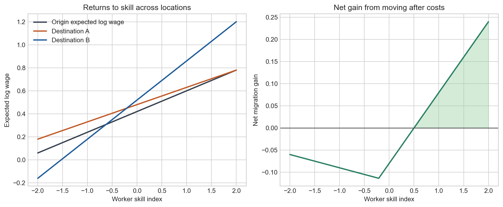
Figure 3:Migration responds to both average wage differences and differential returns to skill. Selection into moving is therefore informative about opportunity sets and moving costs at the same time.
This framework disciplines three common mistakes. First, gross migration rates alone do not reveal whether high-skill workers are sorting toward high-return places. Second, destination wage gains are not automatically causal because movers are selected. Third, place choice is not separable from labor demand, housing, and amenities. Diamond shows why skill groups sort differently across cities when wages, amenities, and housing costs move together Diamond, 2016. Jia, Molloy, Smith, and Wozniak show how much modern internal-migration research is really about labor-market adjustment under heterogeneous local conditions Jia et al., 2023.
Worker mobility and sorting through firms and occupations
Labor economists increasingly ask not just whether workers move, but whether mobility helps them climb wage ladders across employers and occupations. Linked employer-employee panels make that possible because they observe both the worker and the destination firm. The field’s move from cross-sections to matched panels is therefore a conceptual upgrade: mobility can now be analyzed as reallocation across heterogeneous firms rather than as unexplained residual turnover Abowd et al., 1999Card et al., 2013Song et al., 2019.
The core empirical lesson is that firms matter for inequality persistence. If high-income or well-connected workers are more likely to move into high-premium firms, then employer mobility becomes a transmission mechanism for inequality rather than a neutral churn margin. If mobility into better firms is restricted by search frictions, employer practices, or geographic immobility, then wage growth becomes path dependent. This is one reason Week 10 belongs after Week 8 inequality and Week 9 discrimination. Mobility is one channel through which earlier segmentation either relaxes or reproduces itself.
Credit, information, and moving frictions
Moving is costly in a literal sense. Search, transport, deposits, licensing, temporary unemployment, and family disruption all create liquidity and risk problems. That is why a clean lottery object,
is so valuable. Equation (5) asks what happens to labor mobility when access to funds changes for reasons unrelated to workers’ underlying mobility taste or local labor demand. In the credit-lottery setting of Van Doornik et al., 2024, identifying variation comes from quasi-random or randomized financial access rather than from observed mover outcomes alone.
The substantive labor lesson is broader than one paper. Credit frictions can suppress distant job search, reduce willingness to separate from bad current matches, and limit occupational experimentation. Information frictions do something similar even without cash constraints: workers may not know which firms or places offer wage ladders worth the move. Week 11 policy will inherit this logic when it asks whether worker-directed interventions should change incentives, information, or liquidity.
Migration reforms, exposure designs, and labor-market reallocation
Migration also responds to institutional change. A compact exposure-design object is
where indexes region, firm, or worker-market exposure to a migration reform. Equation (6) is not a generic difference-in-differences template pasted onto a labor topic. It is the design logic behind research asking whether new migration access changes firm performance, worker outcomes, or reallocation margins where pre-reform exposure differs Beerli et al., 2021.
The identifying variation must always be stated explicitly. In Beerli, Ruffner, Siegenthaler, and Peri, the relevant variation comes from the abolition of immigration restrictions together with differential pre-reform exposure across firms and markets Beerli et al., 2021. In Foged and Peri, quasi-random dispersal rules create local immigration exposure that is more plausibly exogenous than raw immigrant shares Foged & Peri, 2016. These designs identify reduced-form labor-market responses to migration access. They do not by themselves isolate one pure structural channel because local equilibrium effects, occupational upgrading, and firm responses all move together.
Intergenerational mobility: rank-rank objects and persistence across families
The most common modern summary of intergenerational relative mobility is the rank-rank slope:
where parent and child positions are measured as percentile ranks in their respective income or earnings distributions. A high means stronger persistence and lower relative mobility. The rank-rank object became so influential because it is interpretable, robust to heavy-tailed income distributions, and well suited to administrative data with wide coverage Chetty et al., 2014Acciari et al., 2022.
Transition matrices remain useful companions to Equation (7). A rank-rank slope tells us about average persistence; a quintile transition matrix shows where in the distribution the barriers are tightest. That distinction matters in labor. Upward mobility from the bottom, persistence at the top, and place-specific middle-class stability are different policy and theory problems.
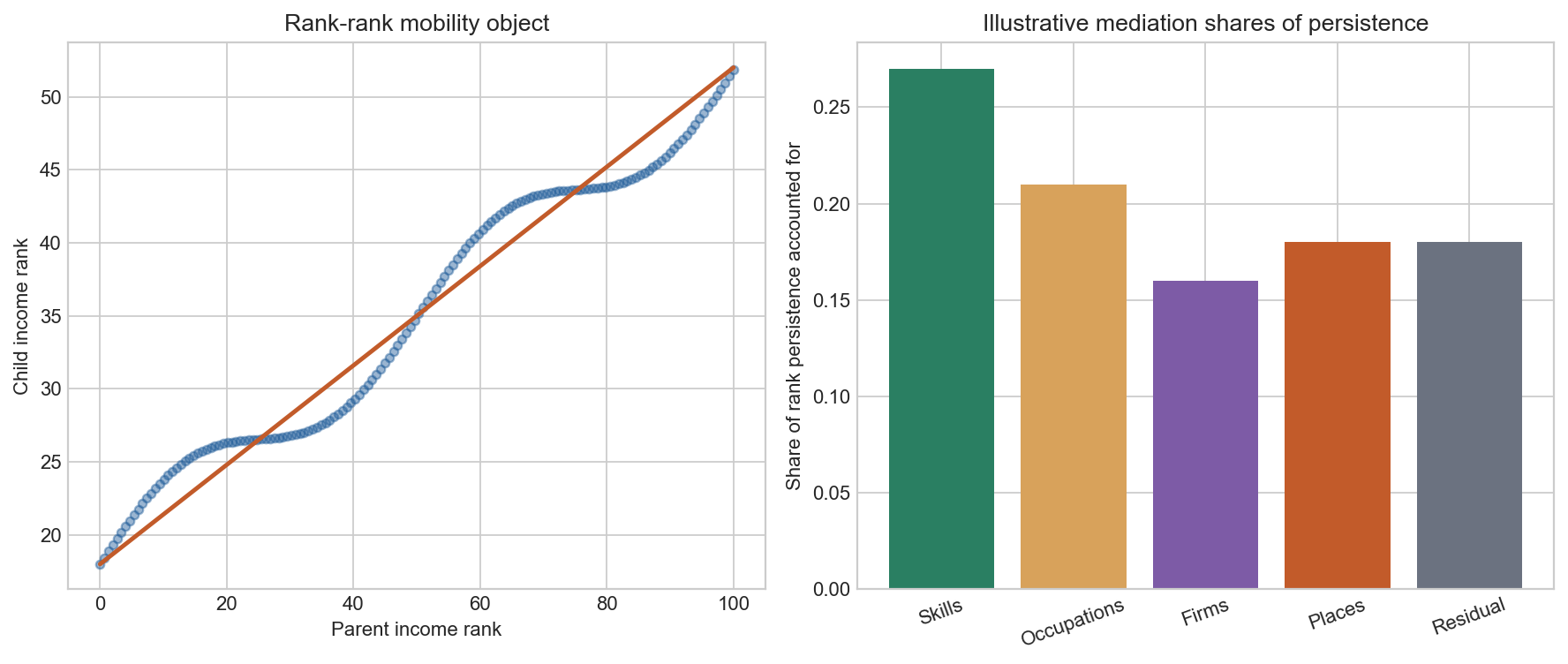
Figure 4:Rank-rank objects summarize persistence, while mediation objects ask which channels carry it. Linked parent-child data made both the descriptive map and the mechanism decomposition substantially more credible.
Linked parent-child administrative data changed the field in the same way linked employer-employee data changed worker mobility research. They reduce classical linkage error, expand geographic coverage, and let researchers map mobility across places and cohorts rather than inferring persistence from small samples Chetty et al., 2014Abramitzky et al., 2021Acciari et al., 2022. But the resulting objects are still descriptive until the researcher makes a mechanism claim.
Table 2:Channels of labor-market transmission across generations
| Channel | Labor-market mechanism | Observable implication | Empirical object |
|---|---|---|---|
| Skills and education | Parents shift children’s human capital and career readiness | Higher earnings rank or faster occupational upgrading | Rank-rank slope, schooling mediation |
| Occupations and careers | Children follow parents into occupations or career ladders | Occupational following and career clustering by parental income | Occupation transition matrix, decomposition by career type |
| Firms and networks | Referrals or firm-specific access shape employer assignment | Higher-quality firm assignment among children from advantaged families | Firm-premium exposure, employer persistence |
| Places and local labor markets | Families sort into locations with different labor demand and wage ladders | Geographic variation in upward mobility and migration responses | Place-level mobility maps, migration selection patterns |
| Information and aspirations | Expectations shape search, moving, and career experimentation | Differential mobility even at similar observed skills | Search or move responses to information or counseling |
| Credit and liquidity | Mobility requires financing search, transport, relocation, or training | Relaxing liquidity constraints increases distant job access | Lottery or credit-access treatment effects |
Table Table 2 lists the main labor-market transmission channels. The key teaching discipline is that “family background” is not itself a mechanism. Skills, occupations, firms, networks, places, information, and credit are mechanisms.
From persistence to mechanism: decomposition and mediation
To move from persistence to mechanism, researchers often study how the parent-rank coefficient changes when a candidate mediator set is introduced:
Equation (8) is not magic causality. It is a disciplined decomposition: shows how much of the parent-rank association is statistically accounted for by channels such as occupation, career path, firm assignment, place, or schooling. Its value is organizational. Its limit is that post-treatment and joint-determination problems remain unless the mediator is itself identified.
That warning matters especially for occupational and career transmission. Haeck and Laliberte show that career structure can account for a meaningful share of intergenerational mobility differences, but the interpretation of a career mediation result still depends on why children enter those careers in the first place Haeck & Laliberté, 2025. Was the driver skill acquisition, neighborhood exposure, licensing barriers, family firms, or information networks? Week 10 should train students to ask that mechanism question before reading a decomposition as a causal answer.
Empirical progress: what the field learned to measure and identify better
Week 10 should explicitly teach empirical progress rather than presenting disconnected findings.
First, linked employer-employee data changed worker mobility from a turnover topic into a firm-sorting topic. Researchers can now separate worker and firm components of wage growth, trace employer-to-employer flows, and study how mobility changes access to high-paying firms Abowd et al., 1999Card et al., 2013Engbom & Moser, 2017.
Second, linked parent-child administrative data changed intergenerational mobility from a small-sample correlation topic into a broad mapping exercise across cohorts, places, and family structures Chetty et al., 2014Abramitzky et al., 2021Acciari et al., 2022.
Third, reform, border, and exposure designs improved migration identification by tying labor-market responses to institutional changes rather than to raw mover comparisons Beerli et al., 2021Foged & Peri, 2016. The identifying variation is not “movers versus stayers”; it is differential exposure to a plausibly exogenous change.
Fourth, lottery-style designs make moving frictions legible by shifting liquidity or access directly Van Doornik et al., 2024. These designs are especially valuable because they speak to whether low mobility reflects preferences or constraints.
Fifth, measurement-correction work matters in its own right. The field improved because it asked whether basic mobility rates were even being measured correctly Fujita et al., 2024.
Finally, rank-rank and transition-matrix approaches improved descriptive clarity. They made mobility patterns easy to compare across places and cohorts, but they must still be paired with mechanism or design work before becoming causal narratives.
Table 3:Methods progression for mobility, migration, and intergenerational transmission
| Design family | Canonical use in this week | What it identifies best | Main threat or limitation |
|---|---|---|---|
| Linked employer-employee panels | Worker mobility, firm sorting, employer wage ladders | Wage changes and reallocation around employer moves | Exogenous-mobility assumptions, measurement of firm identity |
| Measurement-correction designs | Employer-to-employer transition measurement | Corrected mobility series or selection-adjusted flow measures | Dependence on nonresponse or selection-model assumptions |
| Policy reforms / border exposure | Migration and labor-market reallocation after institutional change | Reduced-form effects of migration access on wages, employment, firm outcomes | Concurrent shocks, local equilibrium responses |
| Quasi-random placement rules | Immigration or location exposure based on dispersal rules | Local effects of migration shocks with plausibly exogenous placement | Remaining selection and spillovers |
| Lottery or credit-access designs | Mobility frictions and moving constraints | Causal impact of relaxing mobility constraints | External validity, treatment-takeup margins |
| Rank-rank and transition-matrix methods | Intergenerational mobility measurement | Descriptive persistence and relative mobility patterns | Not a causal mechanism by itself |
| Occupation-based decompositions | Careers and intergenerational persistence | Contribution of occupations/careers to mobility | Descriptive decomposition may not isolate causal channels |
Table Table 3 is the empirical roadmap for the week’s second half. It tells students what each design family identifies well and where it remains vulnerable.
Research Lab
The bounded Week 10 lab follows the standard Reproduce -> Diagnose -> Transfer structure. The reproduction step uses synthetic teaching data in the spirit of Van Doornik et al., 2024 to estimate how randomized credit access changes moving, employer switching, and wage growth. The diagnostic step asks students to explain why this identifies the effect of relaxing a mobility friction rather than the full return to migration. The transfer step then turns to an exposure-design panel in the spirit of Beerli et al., 2021, where students estimate how a migration reform changes local reallocation and worker outcomes in high- versus low-exposure markets.
The local path is deliberately bounded. Students do not need restricted linked employer-employee records or tax-based parent-child data to learn the core logic of Week 10. Optional extensions point them toward Haeck & Laliberté, 2025 for careers and intergenerational persistence and Fujita et al., 2024 for measurement correction in employer-to-employer mobility.
The frontier research questions should stay visible:
When is low mobility efficient persistence in good matches, and when is it trapped labor?
How much of wage growth after a move reflects destination-firm premia, occupation upgrading, or geographic arbitrage?
Which worker-side policies matter most when mobility is limited by credit, information, or housing?
How much of intergenerational persistence operates through firms, occupations, or places rather than schooling alone?
Which descriptive mobility objects are stable enough to guide policy, and which remain sensitive to measurement correction?
Methods Box
Methods Box 1: linked data and measurement correction
Equations (1), (2), and (3) become much more informative once worker and employer records are linked. The gain is not just sample size. It is the ability to observe the destination margin. Measurement-correction work such as Fujita et al., 2024 is part of the same empirical progression because mismeasured employer-to-employer flows distort the basic labor reallocation object before any causal design begins.
Methods Box 2: descriptive mobility versus causal mobility
Equation (7) describes persistence. Equation (8) organizes potential channels. Equation (5) identifies the effect of relaxing one friction. Equation (6) identifies reduced-form responses to a reform with differential exposure. The field improves when students keep those objects separate rather than asking one estimator to answer every mobility question.
Reading Ladder And References
Bridge
Roy on self-selection as an earnings-distribution problem Roy, 1951
Borjas on migrant self-selection Borjas, 1987
Kennan and Walker on expected income and migration choice Kennan & Walker, 2011
Jia, Molloy, Smith, and Wozniak for a modern migration overview Jia et al., 2023
Field Core
Abowd, Kramarz, and Margolis on worker and firm wage components Abowd et al., 1999
Card, Heining, and Kline on workplace heterogeneity and inequality Card et al., 2013
Engbom and Moser on returns to education through access to higher-paying firms Engbom & Moser, 2017
Song, Price, Guvenen, Bloom, and von Wachter on firm-based inequality persistence Song et al., 2019
Beerli, Ruffner, Siegenthaler, and Peri on migration reform and labor-market performance Beerli et al., 2021
Foged and Peri on immigrant exposure and native worker adjustment Foged & Peri, 2016
Chetty, Hendren, Kline, Saez, and Turner on modern intergenerational mobility measurement Chetty et al., 2014
Research Lab
Van Doornik, Gomes, Schoenherr, and Skrastins on credit lotteries and labor mobility Van Doornik et al., 2024
Fujita, Moscarini, and Postel-Vinay on measuring employer-to-employer reallocation Fujita et al., 2024
Abramitzky, Boustan, Jacome, and Perez on intergenerational mobility of immigrants Abramitzky et al., 2021
Acciari, Polo, and Violante on intergenerational mobility in Italy Acciari et al., 2022
Haeck and Laliberte on careers and intergenerational mobility Haeck & Laliberté, 2025
Diamond on skill sorting across places Diamond, 2016
Exercises And Discussion Prompts
Why is a transition matrix like Equation (1) not a causal mobility estimate by itself?
What labor-market question does the hazard object in Equation (2) answer that a transition matrix does not?
In Equation (3), what does the firm-premium term add beyond a generic mover indicator?
Use Equation (4) to explain why destination wage gains among movers need not equal the average treatment effect of moving.
Why can a low migration rate reflect either efficient stability or severe moving frictions?
What is the identifying variation in a credit-lottery design like Equation (5)?
What is the identifying variation in an exposure design like Equation (6)?
Why are rank-rank slopes and quintile transition matrices complements rather than substitutes?
What does Equation (8) teach well, and what does it fail to identify on its own?
How do Week 8 inequality and Week 9 discrimination change the way we should interpret Week 10 mobility evidence?
Which worker-side policies in Week 11 would be most promising if mobility is mainly constrained by credit rather than by preferences?
Reproducibility And Code Lab Note
The Week 10 lab uses a bounded local workflow rather than restricted employer-employee or administrative tax data. Students first reproduce lottery-based mobility effects from a synthetic dataset in the spirit of Van Doornik et al., 2024, then diagnose the identifying margin, and finally transfer the workflow to a migration-reform exposure design in the spirit of Beerli et al., 2021. The student-facing workflow is documented in lab.md.
Slide Companion Note
The Week 10 deck should define mobility as a set of labor-market objects rather than as a single migration statistic. It should bridge directly from Week 9 segmentation, show transition, wage-growth, and rank-rank objects, explain Roy-style migration choice and moving frictions, isolate the logic of lottery and exposure designs, and end by making Week 11 policy look like the study of which frictions are relaxable. The canonical source is 10
Bridge Forward
Use this closing bridge to carry the module’s labor object, mechanism, and evidence into the next course step or research-design exercise.
- Jia, N., Molloy, R., Smith, C., & Wozniak, A. (2023). The Economics of Internal Migration: Advances and Policy Questions. Journal of Economic Literature, 61(1), 144–180. 10.1257/jel.20211623
- Song, J., Price, D. J., Guvenen, F., Bloom, N., & von Wachter, T. (2019). Firming Up Inequality. The Quarterly Journal of Economics, 134(1), 1–50. 10.1093/qje/qjy025
- Chetty, R., Hendren, N., Kline, P., Saez, E., & Turner, N. (2014). Is the United States Still a Land of Opportunity? Recent Trends in Intergenerational Mobility. American Economic Review, 104(5), 141–147. 10.1257/aer.104.5.141
- Diamond, R. (2016). The Determinants and Welfare Implications of US Workers’ Diverging Location Choices by Skill: 1980–2000. American Economic Review, 106(3), 479–524. 10.1257/aer.20131706
- Kennan, J., & Walker, J. R. (2011). The Effect of Expected Income on Individual Migration Decisions. Econometrica, 79(1), 211–251. 10.3982/ECTA4657
- Van Doornik, B., Gomes, A., Schoenherr, D., & Skrastins, J. (2024). Financial Access and Labor Market Outcomes: Evidence from Credit Lotteries. American Economic Review, 114(6), 1854–1881. 10.1257/aer.20230585
- Haeck, C., & Laliberté, J.-W. (2025). Careers and Intergenerational Income Mobility. American Economic Journal: Applied Economics, 17(1), 431–458. 10.1257/app.20230403
- Fujita, S., Moscarini, G., & Postel-Vinay, F. (2024). Measuring Employer-to-Employer Reallocation. American Economic Journal: Macroeconomics, 16(3), 1–51. 10.1257/mac.20210076
- Abowd, J. M., Kramarz, F., & Margolis, D. N. (1999). High Wage Workers and High Wage Firms. Econometrica, 67(2), 251–333. 10.1111/1468-0262.00020
- Card, D., Heining, J., & Kline, P. (2013). Workplace Heterogeneity and the Rise of West German Wage Inequality. The Quarterly Journal of Economics, 128(3), 967–1015. 10.1093/qje/qjt006
- Engbom, N., & Moser, C. (2017). Returns to Education through Access to Higher-Paying Firms: Evidence from US Matched Employer-Employee Data. American Economic Review: Papers and Proceedings, 107(5), 374–378. 10.1257/aer.p20171013
- Roy, A. D. (1951). Some Thoughts on the Distribution of Earnings. Oxford Economic Papers, 3(2), 135–146. 10.1093/oxfordjournals.oep.a041827
- Borjas, G. J. (1987). Self-Selection and the Earnings of Immigrants. American Economic Review, 77(4), 531–553.
- Beerli, A., Ruffner, J., Siegenthaler, M., & Peri, G. (2021). The Abolition of Immigration Restrictions and the Performance of Firms and Workers: Evidence from Switzerland. American Economic Review, 111(3), 976–1012. 10.1257/aer.20181779
- Foged, M., & Peri, G. (2016). Immigrants’ Effect on Native Workers: New Analysis on Longitudinal Data. American Economic Journal: Applied Economics, 8(2), 1–34. 10.1257/app.20150114