Discrimination, Measurement, and Sorting
Learning Objectives
By the end of Week 9, students should be able to:
explain why a raw group gap is not yet a measure of discrimination;
distinguish taste-based discrimination, statistical discrimination, identity or norm-based mechanisms, and sorting or segmentation mechanisms;
explain how discrimination can operate at hiring, wage, promotion, task-assignment, and retention margins;
write down and interpret raw-gap, conditional-gap, decomposition, taste-based, statistical-discrimination, audit, and sorting objects;
explain why omitted variables, post-treatment controls, and endogenous selection complicate empirical measurement;
distinguish what correspondence or audit studies identify from what regression decompositions identify;
connect discrimination to Week 8 inequality without collapsing discrimination into general dispersion;
see why Week 10 mobility is partly about how workers move across labor-market segments that may already be shaped by discrimination.
Opening Orientation
The economic question for the week is narrower and harder than Week 8’s question. Week 8 mapped the architecture of inequality across wages, hours, firms, and amenities. Week 9 asks which part of observed group differences should be interpreted as discrimination, through which mechanism, at which margin, and under which identification design Altonji & Blank, 1999Heckman, 1998Neumark, 2018.
Bridge
Week 8 taught three disciplines that matter immediately here. First, inequality is multi-object: wages, annual earnings, employment, task assignment, and access to high-premium firms can all diverge. Second, descriptive decompositions are useful without being fully causal. Third, sorting across firms and segments is not background noise; it is part of labor-market architecture. Week 9 keeps those disciplines and asks a sharper question: when should unequal labor-market outcomes across groups be read as discrimination rather than as broader inequality?
That sharper question is difficult because observed gaps mix many channels. Group differences in labor outcomes can reflect pre-market skill accumulation, endogenous schooling responses, occupational steering, employer tastes, employer beliefs under imperfect information, unequal access to search networks, and differential assignment across firms, occupations, tasks, and places Becker, 1957Phelps, 1972Arrow, 1973. The field’s core challenge is therefore conceptual and empirical at once. Students must separate gaps from treatment, beliefs from preferences, and within-firm wedges from between-firm allocation.
Field Core
From outcome gaps to discrimination objects
The cleanest opening distinction is between an observed gap and discriminatory treatment. Let index a signaled group identity and let denote a labor-market outcome such as callback probability, hourly wage, promotion, or assignment to a high-contact task. Then the raw gap is
Equation (1) is often the first object the public sees, but it is not yet a discrimination estimate. It is an average difference in outcomes across groups. A conditional analogue,
asks a different question by holding fixed some observed characteristics . The difficulty is that the meaning of Equation (2) depends entirely on what enters . Conditioning on pre-market characteristics can be useful. Conditioning on schooling, occupation, firm assignment, or current task can be dangerous if those variables are themselves downstream of discrimination Altonji & Blank, 1999Heckman, 1998.
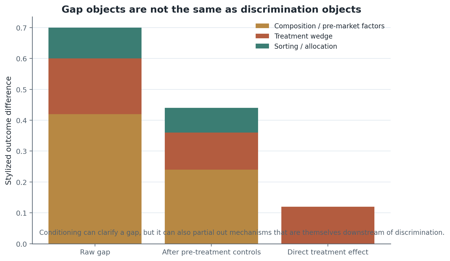
Figure 1:Raw gaps, adjusted gaps, and causal discriminatory treatment are different objects. Conditioning can remove relevant composition differences, but it can also partial out mechanisms that are themselves shaped by discrimination.
Figure Figure 1 should be read as a warning against naive residual reasoning. A raw gap can be too broad to interpret, but a conditional gap can be too narrow if the controls erase the mechanism of interest. Week 9 therefore studies discrimination as an architecture of objects rather than as one residual number.
Competing economic definitions of discrimination
The classic economic definitions remain foundational because they classify mechanisms that often look similar in reduced form.
Taste-based discrimination enters the decision maker’s utility or effective cost function. Becker’s formulation treats group identity as a wedge that makes some workers less attractive to prejudiced employers, coworkers, or customers even when productivity is the same Becker, 1957. Statistical discrimination instead operates through beliefs under imperfect information: employers use group-conditioned expectations when signals about productivity are noisy or incomplete Phelps, 1972Arrow, 1973. Identity, norm, or stigma mechanisms add a broader social layer in which workplace culture, evaluative standards, and interaction effects alter outcomes even without a literal taste parameter or a simple Bayesian signal problem Altonji & Blank, 1999.
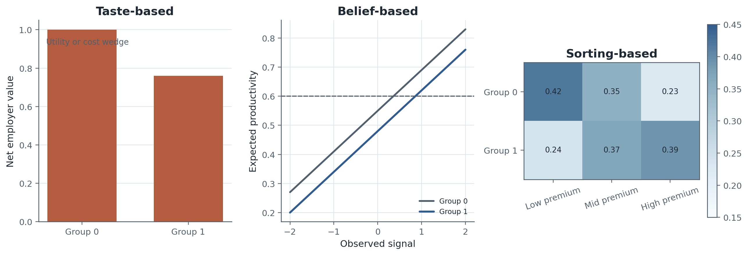
Figure 2:The same observed gap can arise through taste-based wedges, belief-based screening, or allocation-based sorting. The empirical task is to separate mechanisms rather than to assume one canonical channel.
Figure Figure 2 matters because many empirical papers identify treatment differences without pinning down whether the operative channel is taste, beliefs, norms, or equilibrium allocation. Labor economists need the mechanism map before they can decide which estimand is informative.
Table 1:Mechanism map for discrimination research
| Mechanism | Core idea | Main observables | Typical prediction | Main pitfall |
|---|---|---|---|---|
| Taste-based discrimination | Group identity enters utility or effective labor cost | hiring, wages, promotions, segregation | prejudiced decision makers impose a group-specific wedge | competition need not eliminate the wedge at every margin |
| Statistical discrimination | Noisy signals lead employers to use group-conditioned beliefs | callbacks, wages, schooling returns, task assignment | treatment differences appear when signals are incomplete or costly | easy to confuse with omitted productivity measures |
| Identity / norms / stigma | social meaning and workplace norms affect behavior and evaluation | performance ratings, occupations, retention, promotion | identical productivity may be interpreted differently across groups | mechanisms can look like taste or belief discrimination in reduced form |
| Sorting / segmentation | groups are differentially assigned across firms, occupations, tasks, or networks | firm assignment, occupation shares, wage premia, mobility | group gaps persist even without large within-cell treatment effects | hard to separate discrimination from endogenous application or search behavior |
Table Table 1 is the summary map for this section. It keeps the lecture from collapsing into either a history-of-thought survey or an undifferentiated list of discriminatory outcomes.
Measurement architecture: why gaps are not enough
The source pack insists that Week 9 train students to resist turning any conditional residual into “discrimination.” The workhorse descriptive device is still Oaxaca-Blinder style accounting:
Equation (3) is useful because it separates composition differences from coefficient differences. But the second term is not automatically a causal measure of discrimination Altonji & Blank, 1999. Coefficient differences can reflect omitted productivity dimensions, equilibrium responses, measurement error, or selection into the observed sample. The decomposition is descriptive discipline, not a stand-alone identification design.
This is where bad controls enter. Suppose current occupation, firm, or schooling is partly shaped by discriminatory screening earlier in the life cycle. Conditioning on those variables may absorb exactly the mechanism one wants to understand. The same problem arises if the wage sample contains only workers who were hired. Employment selection can turn wage-gap inference into a selected-sample problem: the observed wage gap among workers need not equal the gap that would arise in the full applicant pool Heckman, 1998.
The central habit for students is therefore procedural. Before interpreting a gap, ask:
What is the outcome?
What is the conditioning set?
Which controls are plausibly pre-treatment?
What selection process determines who enters the sample?
Could discrimination at an earlier margin already be hidden inside the observables?
Mechanism block I: taste-based discrimination
The cleanest compact taste-based object is an employer profit function with a group-specific wedge:
In Equation (4), acts like a group-specific cost wedge for employer . Even if worker productivity is identical, prejudiced employers behave as if some workers are more expensive. That can lower hiring, reduce wages, distort task assignment, or push workers toward less prejudiced firms or occupations Becker, 1957.
The important field-course correction is that competition need not wash this away mechanically. Search frictions, customer discrimination, coworker tastes, local concentration, and information frictions can let taste-based wedges survive in equilibrium. Taste-based models therefore predict both treatment differences and sorting patterns. If prejudiced employers avoid certain workers, those workers may be concentrated in particular firms, market segments, or tasks even when within-firm wage gaps look modest.
Mechanism block II: statistical discrimination and belief-based mechanisms
The compact statistical-discrimination object is a group-conditioned decision rule:
Equation (5) says that employers hire when expected productivity , inferred from signals and group identity , exceeds a threshold . The mechanism operates through beliefs rather than tastes. If signals are noisy and employers believe one group has a lower mean or a wider distribution, they may screen differently even when they do not literally dislike the group Phelps, 1972Arrow, 1973.
This mechanism connects directly to Week 4 and Week 5. If workers anticipate that returns to a credential or signal differ by group, then schooling, task acquisition, test-taking, and occupational investment can respond endogenously. Lang and Manove show why education can function as a compensating signal in a discriminatory environment rather than as a clean pre-treatment control Lang & Manove, 2011. That is precisely why Week 9 cannot treat all observed human-capital variables as innocent controls.
Belief-based models also generate feedback. If biased beliefs steer some groups away from high-return tasks or firms, the resulting observed productivity distribution may later appear to validate the original screening rule. This is one route through which discrimination becomes an equilibrium allocation problem rather than just a one-shot hiring decision.
Mechanism block III: discrimination, segmentation, and sorting
Week 9 is the week where discrimination and sorting must be taught together. A compact sorting object is
or, equivalently, the expected premium of the firm to which a worker from group is assigned, . Equation (6) makes the point that discrimination can appear through assignment across firms, occupations, tasks, networks, or local labor markets. It is not only a within-firm wage wedge.
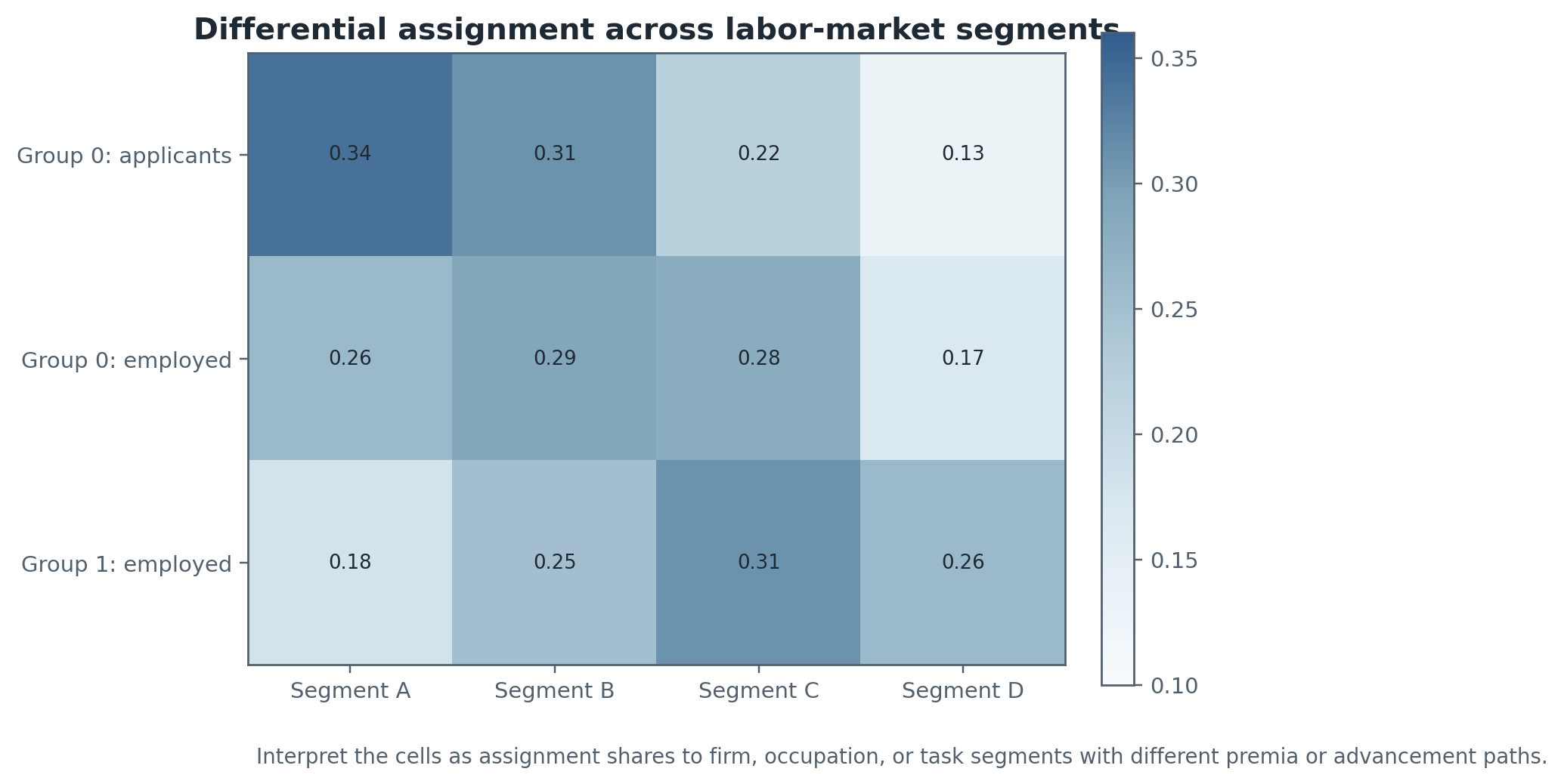
Figure 3:Sorting and segmentation can generate persistent group differences through differential assignment to low-premium and high-premium firms, occupations, or tasks. Observed treatment gaps and allocation gaps often coexist.
Figure Figure 3 is the bridge back to Week 8’s firm and sorting architecture and forward to Week 10 mobility. A worker may face little within-firm wage discrimination conditional on task, yet still be disproportionately sorted into low-premium firms or low-learning tasks. Conversely, large within-firm treatment gaps may coexist with modest between-firm sorting. The empirical lesson is that discriminatory treatment and discriminatory allocation are complements, not substitutes.
Table 2:Sorting and segmentation lenses for Week 9
| Sorting margin | Example question | Why it matters for discrimination | Link to later weeks |
|---|---|---|---|
| Occupation | are groups channeled into different job ladders? | discriminatory assignment can look like skill differences in observed data | Week 10 mobility and migration |
| Firm | do groups end up in lower-premium firms? | between-firm assignment can amplify wage gaps even if within-firm treatment gaps are modest | Labor II monopsony, firms, and institutions |
| Task | are groups steered away from customer-facing or high-contact work? | discriminatory task assignment changes wages, promotion, and learning | behavioral labor and personnel economics |
| Network / referral | do application pools differ because of network access? | hiring gaps can partly reflect unequal access to opportunities generated by past discrimination | Week 11 policy evaluation |
| Location / segment | are groups concentrated in different local or market segments? | segmentation changes outside options and market power | Week 10 place-based mobility |
Table Table 2 keeps the segmentation block concrete. Occupation, firm, task, network, and location margins each generate different empirical objects and different bridges to later weeks.
Empirical identification: what designs identify
The cleanest direct-treatment object in the weekly package comes from correspondence or audit studies:
where treatment changes signaled identity while holding qualifications fixed, and is a callback or contact outcome. Equation (7) is powerful because it makes discriminatory treatment experimentally legible at a specific hiring margin Bertrand & Mullainathan, 2004Neumark, 2018.
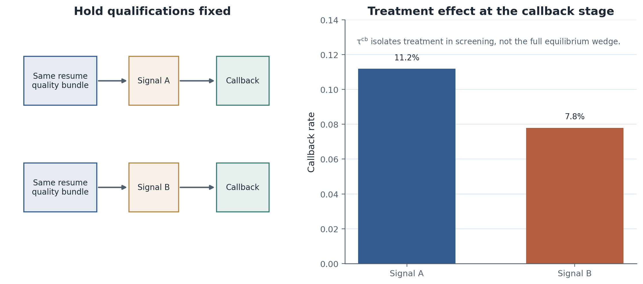
Figure 4:Correspondence and audit studies isolate treatment at a specific margin by changing signaled identity while holding credentials fixed. The design is clean at the callback stage but does not by itself recover every equilibrium consequence of discrimination.
Figure Figure 4 highlights both the strength and the limit of the design. A correspondence experiment identifies a treatment effect in the opportunity set presented to employers. It is especially good for hiring-stage discrimination because it holds application content fixed. But it does not, by itself, reveal the full wage path, task assignment, or equilibrium sorting consequences generated after hiring.
Table 3:Identification map for empirical discrimination designs
| Design | What varies? | Main estimand | Strength | Limitation |
|---|---|---|---|---|
| Oaxaca--Blinder / regression decomposition | conditioning set and coefficient structure | descriptive explained vs unexplained gap | transparent and easy to implement | not fully causal; sensitive to controls and functional form |
| Correspondence / audit study | signaled identity holding credentials fixed | direct treatment effect at callback/contact margin | clean treatment variation | narrow margin; equilibrium consequences not fully observed |
| Paired audits / within-firm comparisons | matched testers or matched applicants | treatment within common opportunity set | controls for some demand heterogeneity | costly, limited external validity, tester effects |
| Quasi-experimental information or policy design | information sets, monitoring, or legal environment | causal change in discriminatory treatment or belief updating | broader institutional insight | design-specific interpretation |
| Structural / equilibrium model | primitives generating wages, task choice, and sorting | inferred discrimination wedge in equilibrium | connects treatment to allocation and welfare | strong modeling assumptions |
Table Table 3 should organize the empirical core of the lecture. Oaxaca-Blinder decompositions answer descriptive accounting questions. Correspondence studies identify treatment at a narrow margin. Paired audits control common opportunity sets more tightly. Quasi-experimental information or policy shocks speak to broader institutional channels. Structural and equilibrium models connect treatment, sorting, and welfare, but at the cost of stronger assumptions Heckman, 1998Neumark, 2018.
How to think about causality in discrimination research
Week 9’s main causal-inference lesson is that the appropriate estimand depends on the mechanism and margin. A callback treatment effect from Equation (7) identifies discriminatory treatment in a specific stage of employer screening. It is not the same as the wage gap among employed workers, because the wage sample is already selected by earlier hiring decisions. A coefficient-difference term in Equation (3) may be informative, but it does not recover a clean treatment effect without much stronger assumptions. A sorting object such as Equation (6) may capture an equilibrium barrier, but it mixes preferences, constraints, search, networks, and employer behavior unless the design separates them.
Heckman’s critique remains essential here. If discrimination affects who applies, who is interviewed, who is hired, and who remains employed, then inference at any later margin inherits the earlier selection problem Heckman, 1998. That is why modern discrimination research often uses a portfolio of designs rather than a single estimator. Experimental designs reveal direct treatment at one stage; decomposition work clarifies how much is left unexplained conditional on chosen controls; structural and equilibrium work translate treatment and sorting into broader labor-market wedges Neumark, 2018Kline et al., 2024Hurst et al., 2024.
The right Week 9 conclusion is therefore disciplined rather than cynical. No single design is enough for every discrimination question, but different designs are informative precisely because they target different objects.
Research Lab
The bounded Week 9 lab follows the standard Reproduce -> Diagnose -> Transfer structure with a teaching-safe path that stays fully local. The reproduction step uses a synthetic correspondence-study file in the spirit of Bertrand & Mullainathan, 2004 to estimate an average callback gap, quality-specific callback gaps, and firm-segment heterogeneity. The diagnostic step asks students to explain why that treatment effect is narrower than a general labor-market discrimination object. The transfer step then moves to synthetic employer-level report cards in the spirit of Kline et al., 2024, where students estimate firm-specific callback gaps, think about noise in rankings, and see how measurement uncertainty complicates employer comparisons.
An optional extension note points to Hurst et al., 2024, where discrimination operates partly through task assignment and equilibrium occupational structure. That extension is deliberately conceptual in the bounded path. Students do not need restricted employer microdata or a real field experiment to learn the core logic of discrimination measurement and sorting.
Open research questions should remain visible:
How much of an observed wage gap reflects treatment at the hiring stage versus sorting across firms and tasks?
When do information frictions and taste-based wedges produce observationally similar patterns?
How much uncertainty should researchers tolerate before ranking employers by discriminatory behavior?
How do discriminatory beliefs alter human-capital investment before workers ever enter the observed labor market?
Which mobility margins in Week 10 reflect voluntary reallocation and which reflect movement within a segmented opportunity set?
Methods Box
Methods Box 1: decomposition discipline and bad controls
Equations (1), (2), and (3) are descriptive tools for organizing group differences. They are most useful when they clarify which part of a gap is tied to observables and when they force the researcher to defend the conditioning set. They become misleading when post-treatment controls are added mechanically or when the unexplained component is relabeled as causal discrimination without a design argument Altonji & Blank, 1999Heckman, 1998.
Methods Box 2: experimental treatment effects, firm report cards, and sorting
Equation (7) gives a sharp experimental object at the callback stage. Equation (6) extends the conversation from direct treatment to equilibrium allocation. Modern firm-level report-card work sits between these objects: it keeps the treatment logic of audits while asking how discrimination varies across firms and how precisely those differences can be estimated Bertrand & Mullainathan, 2004Kline et al., 2024.
Reading Ladder And References
Bridge
Becker on taste-based discrimination Becker, 1957
Phelps and Arrow on statistical discrimination and group-conditioned beliefs Phelps, 1972Arrow, 1973
Field Core
Altonji and Blank for a broad labor-market synthesis of race and gender evidence Altonji & Blank, 1999
Heckman on what audit studies and residual gaps do and do not identify Heckman, 1998
Bertrand and Mullainathan for a transparent experimental treatment-gap design Bertrand & Mullainathan, 2004
Lang and Manove for the interaction between education, signaling, and discrimination Lang & Manove, 2011
Neumark for a modern synthesis of experimental discrimination evidence Neumark, 2018
Research Lab
Kline, Rose, and Walters on employer discrimination report cards and ranking uncertainty Kline et al., 2024
Hurst, Rubinstein, and Shimizu on task-based discrimination and equilibrium occupational assignment Hurst et al., 2024
Exercises And Discussion Prompts
Why does Equation (1) not identify discrimination by itself?
Give one example of a control variable that may be pre-treatment and one that may be post-treatment in a wage-gap regression.
In Equation (3), why is the coefficient-difference term not automatically a clean discrimination measure?
Use Equation (4) to explain why taste-based discrimination can generate both pay gaps and firm segregation.
Use Equation (5) to explain how noisy signals can create discriminatory treatment without employer prejudice in the Becker sense.
Why can education be a bad control in discrimination work if credentials are themselves chosen in anticipation of differential treatment?
What does a correspondence-study estimand like Equation (7) identify especially well, and what does it leave unresolved?
How can Equation (6) help explain persistent group wage gaps even when within-firm wage gaps appear modest?
Which concepts from Week 8 inequality are necessary before a student can interpret Week 9 discrimination evidence carefully?
Why is Week 10 mobility partly about movement across an opportunity set that Week 9 shows may already be segmented?
Reproducibility And Code Lab Note
The Week 9 lab uses a bounded local workflow rather than a literal field-experiment replication. Students first reproduce callback-gap summaries from a synthetic correspondence-study dataset in the spirit of Bertrand & Mullainathan, 2004, then diagnose what that treatment effect does and does not identify, and finally transfer the logic to firm-level discrimination report cards in the spirit of Kline et al., 2024. The student-facing workflow is documented in lab.md.
Slide Companion Note
The Week 9 deck should isolate the chapter’s architecture rather than reproduce its prose. It should start from the Week 8 inequality bridge, define the difference between gaps and discrimination objects, contrast taste-based and statistical-discrimination mechanisms, warn about bad controls, show the logic of audit identification, keep sorting and segmentation inside the discrimination lecture, and end by bridging to Week 10 mobility. The canonical source is 09
Bridge Forward
Use this closing bridge to carry the module’s labor object, mechanism, and evidence into the next course step or research-design exercise.
- Altonji, J. G., & Blank, R. M. (1999). Race and Gender in the Labor Market. In O. Ashenfelter & D. Card (Eds.), Handbook of Labor Economics (Vol. 3C, pp. 3143–3259). Elsevier. 10.1016/S1573-4463(99)30039-0
- Heckman, J. J. (1998). Detecting Discrimination. Journal of Economic Perspectives, 12(2), 101–116. 10.1257/jep.12.2.101
- Neumark, D. (2018). Experimental Research on Labor Market Discrimination. Journal of Economic Literature, 56(3), 799–866. 10.1257/jel.20161309
- Becker, G. S. (1957). The Economics of Discrimination. University of Chicago Press.
- Phelps, E. S. (1972). The Statistical Theory of Racism and Sexism. American Economic Review, 62(4), 659–661.
- Arrow, K. J. (1973). The Theory of Discrimination. In O. Ashenfelter & A. Rees (Eds.), Discrimination in Labor Markets (pp. 3–33). Princeton University Press.
- Kline, P., Rose, E. K., & Walters, C. R. (2024). A Discrimination Report Card. American Economic Review, 114(8), 2472–2525. 10.1257/aer.20230700
- Hurst, E., Rubinstein, Y., & Shimizu, K. (2024). Task-Based Discrimination. American Economic Review, 114(6), 1723–1768. 10.1257/aer.20220234
- Lang, K., & Manove, M. (2011). Education and Labor Market Discrimination. American Economic Review, 101(4), 1467–1496. 10.1257/aer.101.4.1467
- Bertrand, M., & Mullainathan, S. (2004). Are Emily and Greg More Employable Than Lakisha and Jamal? A Field Experiment on Labor Market Discrimination. American Economic Review, 94(4), 991–1013. 10.1257/0002828042002561