Labor Market Facts, Measurement, and Canonical Questions

Learning Objectives¶

By the end of Week 1, students should be able to:

distinguish the core labor-market outcome objects and their measurement units;
explain why labor economists separate stocks from flows, prices from quantities, and levels from composition-adjusted changes;
interpret a compact set of decisive facts on participation, employment, unemployment, hours, wages, earnings, and inequality;
connect those facts to later modules on labor supply, human capital, households, discrimination, firms, frictions, and institutions;
explain why careful description is part of the field’s identification strategy rather than mere background.

Opening Orientation¶

The economic question for the week is simple but foundational: which labor-market facts organize the rest of the labor sequence, and what measurement choices determine how those facts should be interpreted?

Bridge¶

Week 1 starts with objects, not models. Labor economics repeatedly returns to a short list of measured outcomes: employment, unemployment, labor-force participation, hours, hourly wages, weekly earnings, compensation, and transitions across labor-market states. Those objects are small in number, but they already embed big choices about the unit of observation, the relevant denominator, and the institutional rules that determine who appears in a sample.

Four distinctions keep the week disciplined.

Stocks are not flows. The unemployment rate is a stock; job finding and separation are flows.
Prices are not quantities. Hourly wages answer a different question from weekly earnings or hours worked.
Worker outcomes are not firm outcomes. A worker’s wage can move because of skill prices, hours, occupation, employer sorting, or institutions.
Levels are not composition-adjusted changes. An aggregate average can move because the same workers are paid differently or because the mix of observed workers changes.

The practical implication is that labor-market description is already theory-laden. A chapter that says “wages rose” before defining the sample, unit, and weighting rule has not yet said anything precise.

What counts as a labor-market fact?¶

A useful Week 1 fact has three properties. It names a measurable object, it identifies the comparison being made, and it signals what the fact cannot tell us by itself. The employment-population ratio, for example, is not a generic business-cycle statistic. It is a summary of labor-force attachment and successful employment conditional on being in the relevant population.

\frac{E_t}{P_t} = \frac{L_t}{P_t}\left(1-u_t\right)

(1)

Equation (1) is the Week 1 accounting identity. The employment-population ratio combines labor-force participation, $L_t / P_t$ , with the probability of being employed conditional on labor-force attachment, $1-u_t$ . That is why later modules can disagree about mechanisms while still talking about the same observed series. A fall in $E_t/P_t$ may come from weaker participation, weaker job finding, or both.

A first empirical dashboard¶

U.S. labor-market status dashboard using public FRED series for the labor-force participation rate (CIVPART), employment-population ratio (EMRATIO), and unemployment rate (UNRATE) from 1976 forward. The unemployment rate is plotted on a secondary axis. The point of the figure is that participation, employment, and unemployment are related but non-identical indicators, so descriptive work must name the object before moving to mechanism. 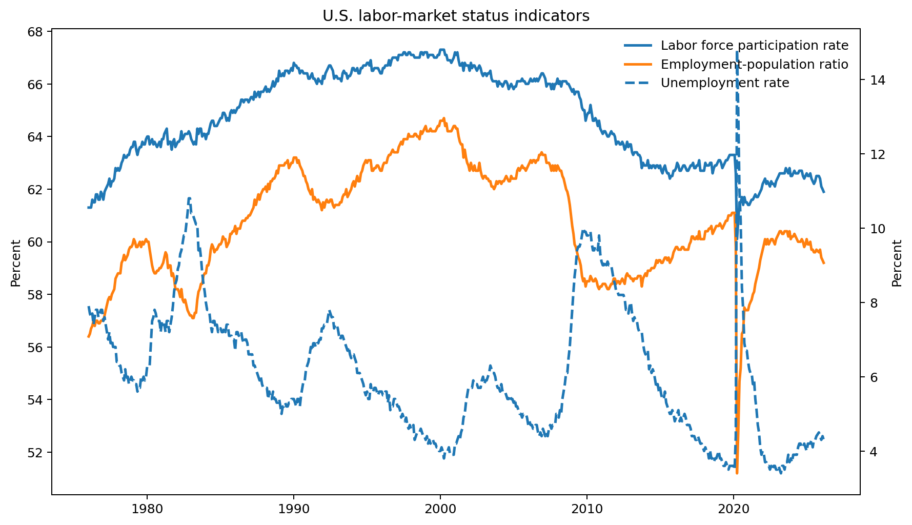— Figure 1:U.S. labor-market status dashboard using public FRED series for the labor-force participation rate (`CIVPART`), employment-population ratio (`EMRATIO`), and unemployment rate (`UNRATE`) from 1976 forward. The unemployment rate is plotted on a secondary axis. The point of the figure is that participation, employment, and unemployment are related but non-identical indicators, so descriptive work must name the object before moving to mechanism.

Figure Figure 1 is intentionally introductory. The substantive lesson is not the level of the synthetic series. It is that three indicators that students often collapse into “the labor market” answer different questions, and the accounting identity in Equation (1) explains why.

Field Core¶

Measurement architecture¶

The Current Population Survey is the workhorse U.S. source for labor-force status, hours, and many earnings objects used in field-course teaching and empirical labor research. That statement is less trivial than it sounds. The CPS gives the field a common language for employment, unemployment, nonparticipation, demographic subgroups, and many earnings comparisons, which is why the rest of the course can reuse Week 1 definitions rather than reinvent them each week.

The key measurement objects appear in Table Table 1.

Table 1:Measurement map for recurring Week 1 objects.

Object	Economic meaning	Typical unit of observation	Common U.S. source	Common analytical use
Employment	Whether an individual worked or held a job in the reference period	Person-month or person-quarter	CPS	Participation, cyclicality, subgroup gaps
Unemployment	Non-employment among active searchers	Person-month	CPS	Slack, job-finding conditions, policy response
Labor-force participation	Whether an individual is in the labor force	Person-month	CPS	Extensive-margin labor supply, attachment, lifecycle analysis
Hours worked	Quantity of labor supplied conditional on work	Worker-week or worker-year	CPS, ACS, time-use surveys	Intensive-margin labor supply, earnings decomposition
Hourly wage	Price of labor per hour	Worker-job or worker-week	CPS ORG, survey microdata	Wage-setting, returns to skill, gaps
Weekly earnings	Joint outcome of wages and hours	Worker-week	CPS earnings supplement or ORG-based releases	Distributional facts, group comparisons, worker welfare
Compensation	Wage plus nonwage benefits and employer costs	Job, establishment, or worker-job	Employer surveys, linked data	Incidence, benefits, total rewards
Worker transitions	Movement across employment, unemployment, nonparticipation, jobs, and firms	Person-month panel or linked records	CPS matched files, LEHD, administrative data	Flows, mobility, frictions, scarring

Week 1 uses that table to separate measurement from interpretation. Employment and participation speak to attachment at the extensive margin. Hours and earnings separate intensive-margin behavior from price effects. Compensation reminds students that wages are not the full reward to work. Transitions warn us that a static cross section is often the wrong object for questions about frictions, scarring, or mobility.

Organizing stylized facts¶

The opening labor facts are more coherent when organized around four themes rather than presented as a list.

First, participation and work attachment are highly heterogeneous across demographic groups and the life cycle. Later labor-supply and household modules reuse this fact repeatedly because the key margin is often entry, exit, or hours conditional on work rather than the wage alone.

Second, observed wage and earnings dispersion bundle together prices and composition. A cross-sectional change in mean weekly earnings can reflect changing hours, changing hourly pay, or changing shares of workers in different cells. This is the precise bridge from Week 1 description to later inequality and human-capital modules.

Third, inequality facts are not self-interpreting. A widening distribution can be consistent with shifts in demand, shifts in worker composition, institutional changes, firm effects, or some combination. Week 1 does not settle the mechanism; it defines the object that later weeks try to explain.

Fourth, group gaps cannot be treated as pure worker-characteristic gaps. Occupations, firms, job ladders, bargaining environments, and policy institutions shape the measured outcomes. That is why Labor I begins with worker-side objects but cannot remain worker-only for long.

Composition, aggregation, and the Week 1 lab¶

The lab anchors the chapter’s second formal object.

\Delta \bar{w}_t = \sum_g \left(s_{gt} - s_{g,t-1}\right)\bar{w}_{g,t-1} + \sum_g s_{g,t-1}\left(\bar{w}_{gt} - \bar{w}_{g,t-1}\right) + R_t

(2)

Equation (2) separates aggregate wage change into a composition term, a within-group wage term, and a remainder from using a discrete-time decomposition. The first term asks whether the observed workforce became more concentrated in higher- or lower-wage cells. The second asks whether wages changed within those cells. This is the accounting logic behind the Daly-Hobijn exercise in the Week 1 lab.

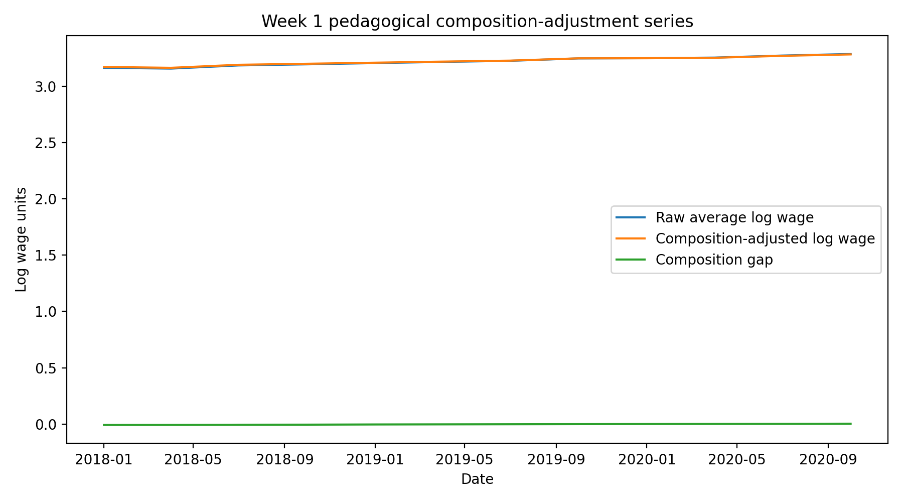
Figure 2:Reduced pedagogical reproduction of the Week 1 composition-adjustment exercise. The raw series, composition-adjusted series, and composition gap are constructed from the teaching panel used in the local lab workflow. The figure shows why aggregate wage growth cannot be read as a pure price series without checking who is observed in employment.

The connection between Equations (1) and (2) is the core intellectual move of the week. The first decomposes work attachment into participation and conditional employment. The second decomposes aggregate pay into a changing workforce mix and within-cell wage movements. Both warn against treating a top-line aggregate as a mechanism.

Week 1 facts as inputs to later modules¶

Table 2:How Week 1 objects reappear later in the sequence.

Week 1 object or fact	Later module(s)	Why it returns
Employment-population ratio versus unemployment	Labor supply; Labor II aggregate adjustment	Distinguishes participation from job finding
Weekly earnings versus hourly wages	Human capital; inequality; discrimination	Separates price effects from hours and composition
Group heterogeneity in participation and pay	Households; gender; discrimination; mobility	Motivates subgroup analysis and mechanisms
Composition-adjusted versus raw wage growth	Policy evaluation; business cycles; code labs	Reminds students that aggregates can move because the composition of workers changes
Data source choice (CPS, earnings releases, linked employer-employee data)	Methods course; Labor II firm-side modules	Measurement determines what questions can be answered credibly

Table Table 2 is the course map. Week 2 labor supply returns to participation and hours. Human-capital weeks return to wage and earnings measurement. Household and gender weeks return to participation, hours, and group gaps. Labor II returns to the same measured objects from the side of firms, frictions, wage-setting, and institutions.

Research Lab¶

Week 1 is introductory in pacing but not in ambition. The frontier questions already appear once we define the objects carefully.

One frontier question is whether the field’s canonical facts are stable or historically contingent. Participation, unemployment, and earnings dispersion are not timeless constants; they depend on technology, demographics, policy, and market structure.

A second frontier question is how to measure newer forms of work and compensation. Platform work, variable schedules, benefits outside cash wages, and hybrid employment relationships all stress the standard categories that introductory courses take for granted.

A third frontier question is which source of heterogeneity matters most for inequality and mobility: workers, occupations, firms, places, or institutions. Week 1 does not adjudicate that debate, but it equips students to see why the answer cannot be inferred from a single aggregate.

Research extensions for strong students should stay bounded. Reasonable Week 1 extensions include a subgroup factbook by education or sex, a comparison of raw and composition-adjusted wage movements across two episodes, or a short note on how firm-side data would change the interpretation of a worker-side fact.

Methods Box¶

Week 1 introduces a workflow that will recur all semester.

Define the object precisely.
State the unit of observation and denominator.
Separate measurement from mechanism.
Ask whether the aggregate mixes together composition and within-group change.
Only then move to causal or equilibrium claims.

That workflow is why descriptive labor economics is part of identification. A weak definition of the outcome creates a weak empirical design no matter how sophisticated the later estimator appears.

Reading Ladder And References¶

Bridge¶

Labor-market object map from the Week 1 source pack
Introductory CPS documentation and earnings concepts

Field Core¶

Katz and Murphy on wage structure and skill demand
Juhn, Murphy, and Pierce on wage inequality decomposition
Acemoglu and Autor on tasks, skills, and labor-market inequality
Blau and Kahn on gender gaps
Card, Cardoso, Heining, and Kline on firms and inequality

Research Lab¶

Daly and Hobijn on composition and aggregate wage growth
Linked worker-firm and measurement papers assigned later in the sequence

The local bibliography file is currently only a placeholder, so the chapter frontmatter points to the shared BibTeX location but formal citation rendering remains blocked until entries are populated there.

Exercises And Discussion Prompts¶

Why is the employment-population ratio often more informative than the unemployment rate when participation is moving?
Give one labor-market question for which weekly earnings are the wrong outcome and hourly wages are the right one.
In Equation (2), describe one economic event that would primarily move the composition term and one that would primarily move the within-group term.
Choose one Week 1 fact and explain what additional data would be needed to distinguish worker, firm, and institutional mechanisms.

Reproducibility And Code Lab Note¶

The Week 1 lab is a reproduce-and-transfer exercise built around Daly and Hobijn’s composition-adjustment logic. Students first reproduce a bounded descriptive result using the reduced pedagogical dataset and scripts in labs/01-labor-market-facts/src/. They then transfer the same accounting logic to one compact subgroup factbook. The key constraint is that the transfer exercise must preserve the Week 1 object definition rather than drift into an unrelated research project.

Slide Companion Note¶

The slide deck should do less than the chapter and do it more sharply. It should define the week’s central question, show the measurement map, visualize labor-market status, present Equations (1) and (2), and end by showing where these objects return later in Labor I and Labor II.

Bridge Forward¶

Use this closing bridge to carry the module’s labor object, mechanism, and evidence into the next course step or research-design exercise.