Dynamic Labor Supply and Lifecycle Responses
Learning Objectives
By the end of Week 3, students should be able to:
write down a dynamic labor-supply problem with savings and a nonlinear tax schedule;
explain why temporary and permanent wage changes identify different labor-supply objects;
interpret the Frisch elasticity as an intertemporal substitution object rather than a generic elasticity;
connect lifecycle hours and participation profiles to human capital, family timing, and health;
distinguish persistence driven by state dependence or adjustment costs from persistence driven by slow-moving heterogeneity;
explain why dynamic evidence from experiments, panel variation, tax reforms, and lifecycle structural models should not be forced into one elasticity number.
Opening Orientation
The economic question for the week is direct: once work decisions are linked across periods through savings, anticipated wages, taxes, and changing constraints, what exactly does labor-supply evidence identify?
Bridge
Week 2 gave the static first-order condition that maps the net-of-tax wage into a contemporaneous labor-leisure tradeoff. That benchmark remains useful, but it is no longer sufficient once incentives are dynamic. Workers do not encounter taxes, wages, childbearing, health shocks, or retirement decisions as one-shot events. They face timing problems. A temporary bonus today is not the same object as a permanent wage increase, and an anticipated tax holiday is not the same object as an unexpected shift in labor demand Blundell & MaCurdy, 1999Keane, 2011.
The reason is simple but important. In a dynamic environment, current work changes not only current consumption but also assets, future labor choices, and sometimes future wages. The shadow value of wealth is therefore an intertemporal state variable rather than a static constant. That is why dynamic labor-supply evidence is valuable and hard to read at the same time: different designs load differently on intertemporal substitution, wealth effects, and persistence MaCurdy, 1981Chetty, 2012.
Dynamic benchmark
The clean benchmark extends Week 2 by letting the worker choose consumption, hours, and savings over time:
Equation (1) nests the static problem inside a larger intertemporal choice problem. Hours still trade off against leisure, but the payoff to current work depends on how the worker values future resources. That is the sense in which Week 2 survives inside Week 3: the static condition remains on the page, but its interpretation changes because the relevant marginal utility of wealth is now dynamic MaCurdy, 1981Blundell & MaCurdy, 1999.
If the worker is interior within the period, the intratemporal condition can still be written as
Equation (2) looks familiar, but the empirical interpretation is not the same as in Week 2. The Frisch elasticity is the response of hours to a wage change holding fixed the marginal utility of wealth, or equivalently the multiplier on the intertemporal budget constraint. It is therefore a conditional intertemporal substitution object, not the same thing as a static uncompensated elasticity MaCurdy, 1981Keane, 2011.
That distinction matters immediately for temporary versus permanent wage changes. A temporary high wage mainly changes the relative price of leisure across dates, so the clean prediction emphasizes retiming of work effort toward the high-wage period. A permanent wage increase instead brings both substitution and wealth effects, which is why it cannot be read as a pure Frisch object. Once observed responses are small, we still need one more question: is the true substitution motive weak, or are adjustment frictions muting what we see Fehr & Goette, 2007Chetty, 2012?
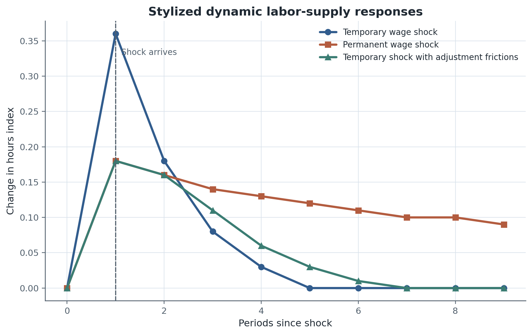
Figure 1:Stylized hours responses to temporary and permanent wage changes. The temporary shock produces a sharper short-run response because it mainly loads on intertemporal substitution. The permanent shock mixes substitution and wealth effects, while adjustment frictions smooth the measured response even when the incentive change is immediate. The figure is conceptual but organized around the distinctions emphasized in Fehr & Goette (2007), Chetty (2012), and Chetty et al. (2011).
Figure Figure 1 summarizes the central Week 3 intuition. Horizon and anticipation are not details to append after estimating an elasticity. They are part of the estimand itself.
Field Core
Lifecycle labor supply and the bridge to human capital
The lifecycle view asks workers to choose not only how much to work, but when. Hours and participation profiles over age are equilibrium objects shaped by wages, assets, family timing, health, and anticipated future returns to work. A rising wage path early in life can raise current labor supply because experience accumulation makes current hours more valuable tomorrow. That is why the line between labor supply and human-capital investment begins to blur in dynamic models Imai & Keane, 2004Attanasio et al., 2008.
This is the crucial bridge into Week 4. Once current work affects future wages through learning-by-doing or experience accumulation, labor supply is no longer only about trading leisure for consumption. It also becomes a decision about when to invest in one’s own productive capacity. Human capital is therefore not a separate topic pasted onto labor supply later in the course; it is already latent inside lifecycle work decisions Imai & Keane, 2004Goldin & Mitchell, 2017.
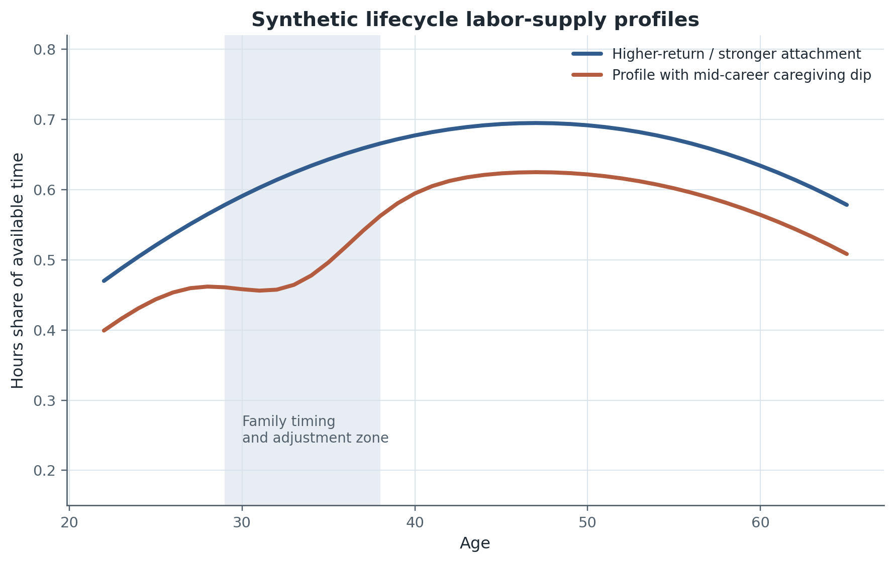
Figure 2:Synthetic lifecycle labor-supply profiles. The profiles are schematic rather than data-cleaned estimates, but they are built to highlight the timing logic in lifecycle labor supply: early-career wage growth can raise hours through future returns, family transitions can create mid-career divergence, and later-life hours reflect both incentives and health or retirement constraints. The motivating empirical backdrop comes from Attanasio et al. (2008), Goldin & Mitchell (2017), and Hokayem & Ziliak (2014).
Figure Figure 2 should be read as a timing map rather than as a descriptive fact to memorize. Female lifecycle employment profiles changed because wages, fertility timing, and household organization changed, not because one static preference parameter was suddenly different Attanasio et al., 2008Goldin & Mitchell, 2017. Health also enters the same lifecycle problem by changing both the utility cost of work and the returns to remaining attached Hokayem & Ziliak, 2014.
Blundell, Pistaferri, and Saporta-Eksten show why the family dimension matters for dynamic interpretation. Consumption smoothing and family labor supply jointly determine whether wage risk turns into hour adjustment, spousal adjustment, or asset decumulation Blundell et al., 2016. That makes lifecycle labor supply empirically inseparable from household structure even before Labor I reaches the dedicated family module.
What dynamic empirical designs identify
The literature is easiest to organize by identifying design rather than chronology.
Table 1:Dynamic labor-supply shock-response taxonomy
| Shock type | Likely primary margin | Object most closely targeted | Main interpretation risk |
|---|---|---|---|
| Temporary unanticipated wage shock | Intensive hours / effort timing | Frisch or intertemporal substitution response | Measured response can be damped by adjustment costs or constraints |
| Temporary anticipated tax holiday | Timing of earnings and hours | Intertemporal substitution with anticipation | Bunching or retiming can overstate broader welfare-relevant labor-supply change |
| Permanent wage change | Hours, participation, career timing | Mix of substitution and wealth effects | Cannot be interpreted as a pure Frisch elasticity |
| Lifecycle wage growth | Hours profile over age | Lifecycle timing under evolving returns to work | Human-capital accumulation and family transitions confound pure labor-supply interpretation |
| One-time fixed work-cost shock | Participation / entry-exit | Extensive-margin threshold response | Persistence after the shock may reflect hysteresis or state dependence |
Table Table 1 is the shortest route from incentive change to target parameter. A temporary unanticipated wage shock is closest to a Frisch or intertemporal substitution response. A permanent wage change mixes substitution and wealth effects. A fixed work-cost shock is often primarily extensive-margin. Lifecycle wage growth is informative about timing but is not a clean primitive unless human capital and family transitions are modeled explicitly Keane, 2011Chetty, 2012.
Table 2:Empirical design map for dynamic labor supply
| Design | Key identifying variation | Object learned | Major threat |
|---|---|---|---|
| Randomized temporary wage variation | Exogenous short-run change in pay | Intertemporal substitution / short-run effort response | External validity to broader labor-market settings |
| Panel wage-hours variation | Within-worker changes in wages and hours over time | Dynamic reduced-form hours response | Wage endogeneity, measurement error, serial correlation |
| Tax timing or tax reform design | Changes in the timing or slope of the net-of-tax schedule | Timing response and horizon-specific elasticities | Anticipation, salience, nonlinear budget-set complexity |
| Lifecycle structural model | Joint restrictions across wages, hours, savings, and family states | Lifecycle labor-supply parameters and counterfactual policy effects | Model dependence and misspecification |
| Event study around a life transition | Discrete timing of childbirth, health shock, or retirement | Persistence and transition dynamics | Concurrent shocks, selection into transition timing |
Table Table 2 turns that logic into an evidence map. Randomized temporary wage variation, such as the experiment in Fehr & Goette, 2007, is attractive because it isolates short-run substitution incentives. Tax timing reforms or nonlinear schedule changes are useful because they create horizon-specific changes in the net reward to work, but anticipation and salience matter immediately Chetty, 2012. Panel wage-hours variation can recover dynamic reduced-form responses, yet only after taking wage endogeneity and serial correlation seriously MaCurdy, 1981. Structural lifecycle models ask more of the reader, but they are often the only way to carry savings, family timing, and human-capital accumulation into policy counterfactuals Attanasio et al., 2008Keane, 2011.
The practical teaching lesson is that two papers can disagree numerically without disagreeing economically. One may target short-run intertemporal substitution. Another may target a long-run policy response after assets, spouses, fertility, and experience have adjusted. Dynamic labor supply becomes useful precisely when we stop forcing those objects into one statistic.
Persistence, state dependence, and adjustment costs
Observed hours often move more slowly than the clean frictionless benchmark suggests. That is not evidence by itself that preferences are flat. It may instead reflect work-schedule rigidities, participation costs, information frictions, institutional constraints, or genuine state dependence in habits and attachment Chetty, 2012Chetty et al., 2011.
One transparent way to formalize this point is to add an adjustment-cost term:
Equation (3) says that changing hours is itself costly. Even when Equation (2) suggests a strong contemporaneous incentive to reoptimize, a large slows the observed response. That interpretation is central to the micro-versus-macro elasticity discussion in Chetty et al., 2011. Short-run administrative or firm-level data may reveal limited immediate adjustment even when longer-run responses after renegotiation or job mobility are larger.
The same logic keeps Week 3 connected to later parts of the course. Adjustment costs and entry-exit costs forecast the household timing issues of Week 6, the horizon problems in Week 11 policy evaluation, and the broader friction-based interpretation of Week 12. Persistence in hours or participation is therefore not a nuisance pattern to difference away. It is itself part of the labor-supply problem.
Research Lab
The frontier challenge is not writing down a dynamic problem. It is deciding which margins need to be in the model before the counterfactual becomes credible. The more the labor-supply path depends on family timing, health, or human-capital accumulation, the less informative a one-period elasticity will be for persistent policy design Attanasio et al., 2008Hokayem & Ziliak, 2014.
This is why dynamic evidence is both powerful and fragmented. Randomized temporary wage variation gives clean leverage on intertemporal substitution but says less about lifecycle family labor supply. Lifecycle structural estimation can speak to richer policy questions but imports stronger assumptions. Tax timing designs sit in the middle: close to policy, but often vulnerable to anticipation, salience, and schedule complexity Fehr & Goette, 2007Chetty, 2012.
The open research agenda follows directly. Which persistence is structural and which is institutional? When do household responses amplify or mute worker-level substitution? Which dynamic objects transport across occupations, countries, or tax systems? Those are the questions that carry Week 3 forward into human capital, family labor supply, and worker-side policy evaluation.
Methods Box
Week 3 adds one discipline to the Week 2 workflow: identify the horizon before interpreting the estimate.
Write the dynamic problem and identify the state variables, especially assets and lagged labor-market choices.
Ask whether the design changes the wage temporarily, permanently, or in an anticipated way.
Decide whether the estimate is closest to a Frisch object, a mixed substitution-and-wealth object, or a persistence object.
Check whether lifecycle features such as experience, family timing, or health make current labor supply affect future opportunities.
Interpret small short-run responses against Equations (2) and (3) before concluding that labor supply is inelastic.
Reading Ladder And References
Bridge
MaCurdy on labor supply in a lifecycle setting and the original Frisch logic MaCurdy, 1981
Blundell and MaCurdy on how static, intertemporal, and lifecycle labor-supply objects differ Blundell & MaCurdy, 1999
Field Core
Keane’s survey on taxes, dynamic labor supply, and why elasticity definitions matter Keane, 2011
Fehr and Goette on randomized temporary wage variation and short-run intertemporal substitution Fehr & Goette, 2007
Attanasio, Low, and Sanchez-Marcos on lifecycle female labor supply and the role of changing returns and family timing Attanasio et al., 2008
Chetty, Friedman, Olsen, and Pistaferri on adjustment costs and micro versus macro elasticities Chetty et al., 2011
Research Lab
Imai and Keane on intertemporal labor supply with human-capital accumulation Imai & Keane, 2004
Blundell, Pistaferri, and Saporta-Eksten on consumption risk and family labor supply Blundell et al., 2016
Goldin and Mitchell on changing lifecycle employment profiles Goldin & Mitchell, 2017
Hokayem and Ziliak on health, human capital, and lifecycle labor supply Hokayem & Ziliak, 2014
Chetty on how optimization frictions reconcile different elasticity estimates Chetty, 2012
Exercises And Discussion Prompts
Use Equations (1) and (2) to explain why a temporary wage shock is closer to a Frisch experiment than a permanent wage increase.
Figure Figure 1 shows a muted short-run response under adjustment frictions. What empirical patterns would help you distinguish a high adjustment cost from a low underlying substitution motive?
In Figure Figure 2, why can a hump-shaped hours profile reflect changing returns to work rather than changing tastes for leisure alone?
Pick one row from Table Table 2 and explain what policy question it can answer well and what policy question it answers poorly.
How does the Week 3 dynamic interpretation change the way you would read static tax-reform evidence from Week 2?
Reproducibility And Code Lab Note
The Week 3 lab is built around a bounded pedagogical version of Fehr & Goette, 2007. Students reproduce one reduced-form response to randomized temporary wage variation using local synthetic shift-level data, diagnose whether that response is best read as intertemporal substitution or something broader, and then transfer the workflow to a persistence comparison that contrasts low- and high-adjustment-cost environments. The optional lifecycle extension uses Attanasio et al., 2008 as the conceptual bridge from short-run experimental variation to lifecycle profile construction. The bounded path and smoke test are documented in lab.md.
Slide Companion Note
The Week 3 deck should isolate the dynamic problem, the Frisch interpretation, the temporary-versus-permanent distinction, the lifecycle profile, the design map, and the adjustment-cost bridge to Week 4 rather than duplicating the chapter. The canonical source is 03
Bridge Forward
Use this closing bridge to carry the module’s labor object, mechanism, and evidence into the next course step or research-design exercise.
- Blundell, R., & MaCurdy, T. (1999). Labor Supply: A Review of Alternative Approaches. In O. Ashenfelter & D. Card (Eds.), Handbook of Labor Economics (Vol. 3A, pp. 1559–1695). Elsevier. 10.1016/S1573-4463(99)03008-4
- Keane, M. P. (2011). Labor Supply and Taxes: A Survey. Journal of Economic Literature, 49(4), 961–1075. 10.1257/jel.49.4.961
- MaCurdy, T. E. (1981). An Empirical Model of Labor Supply in a Life-Cycle Setting. Journal of Political Economy, 89(6), 1059–1085. 10.1086/261024
- Chetty, R. (2012). Bounds on Elasticities with Optimization Frictions: A Synthesis of Micro and Macro Evidence on Labor Supply. Econometrica, 80(3), 969–1018. 10.3982/ECTA9046
- Fehr, E., & Goette, L. (2007). Do Workers Work More if Wages Are High? Evidence from a Randomized Field Experiment. American Economic Review, 97(1), 298–317. 10.1257/aer.97.1.298
- Chetty, R., Friedman, J. N., Olsen, T., & Pistaferri, L. (2011). Adjustment Costs, Firm Responses, and Micro versus Macro Labor Supply Elasticities: Evidence from Danish Tax Records. The Quarterly Journal of Economics, 126(2), 749–804. 10.1093/qje/qjr013
- Imai, S., & Keane, M. P. (2004). Intertemporal Labor Supply and Human Capital Accumulation. International Economic Review, 45(2), 601–641. 10.1111/j.0020-6598.2004.00290.x
- Attanasio, O., Low, H., & Sánchez-Marcos, V. (2008). Explaining Changes in Female Labor Supply in a Life-Cycle Model. American Economic Review, 98(4), 1517–1552. 10.1257/aer.98.4.1517
- Goldin, C., & Mitchell, J. (2017). The New Life Cycle of Women’s Employment: Disappearing Humps, Sagging Middles, Expanding Tops. Journal of Economic Perspectives, 31(1), 161–182. 10.1257/jep.31.1.161
- Hokayem, C., & Ziliak, J. P. (2014). Health, Human Capital, and Life Cycle Labor Supply. American Economic Review: Papers & Proceedings, 104(5), 127–131. 10.1257/aer.104.5.127
- Blundell, R., Pistaferri, L., & Saporta-Eksten, I. (2016). Consumption Inequality and Family Labor Supply. American Economic Review, 106(2), 387–435. 10.1257/aer.20121417