Job Amenities and Compensating Differentials
Learning Objectives
By the end of Week 7, students should be able to:
define compensating differentials and explain why they are equilibrium objects rather than simple wage premia;
write down a worker-side utility object over wages and amenities and interpret the equalizing-differentials condition;
explain why firms choose amenity bundles jointly with wages rather than taking nonwage conditions as fixed background features;
distinguish classic hedonic and risk-premium evidence from modern discrete-choice and revealed-preference approaches;
explain why cross-sectional hedonic wage regressions can fail under sorting, frictions, multidimensional amenities, or mismeasurement;
connect schedule control, remote work, commute burden, safety, and autonomy to a single wage-plus-amenity framework;
distinguish wage inequality from inequality in total job value;
explain why Week 8 inequality and Week 9 discrimination or segmentation must track job quality as well as wages.
Opening Orientation
The economic question for the week is direct: if Week 5 treated wages as a central market outcome and Week 6 showed how households transform wage opportunities into realized labor supply, why do two jobs paying the same wage often represent very different labor-market opportunities once schedule control, safety, commute burden, remote work, and workplace design enter the bundle Rosen, 1986Mas & Pallais, 2017Maestas et al., 2023?
Bridge
Week 5 taught students to treat wages as incomplete objects: measured pay reflects productive skill, selection, sorting, and sometimes rents. Week 6 then showed that households convert wage opportunities into realized hours, participation, and career paths. Week 7 adds a further correction. Workers do not choose wages in the abstract. They choose jobs, and jobs are bundles of pay plus working conditions.
That adjustment is not cosmetic. A high-wage job with an unpredictable schedule, long commute, or injury risk can yield lower worker welfare than a lower-wage job with safety, autonomy, and control over time. Once that is true, observed wage gaps are not automatically welfare gaps, and measured inequality may change once nonwage compensation is counted. This is exactly why compensating differentials belong in the core of labor economics rather than at its margins Hamermesh, 1999Mas & Pallais, 2017.
Jobs are wage-plus-amenity bundles
The clean worker-side object is an indirect-utility representation:
where is the wage and is an amenity index that can summarize safety, schedule predictability, remote work, autonomy, or another nonwage job attribute. If is a good, such as flexibility or safety, then ; if is a bad, such as risk or schedule unpredictability, the same framework can be written with the opposite sign or with a transformed disamenity index. Equation (1) is deliberately compact, but it makes the central point visible: wages are only one argument in worker welfare.
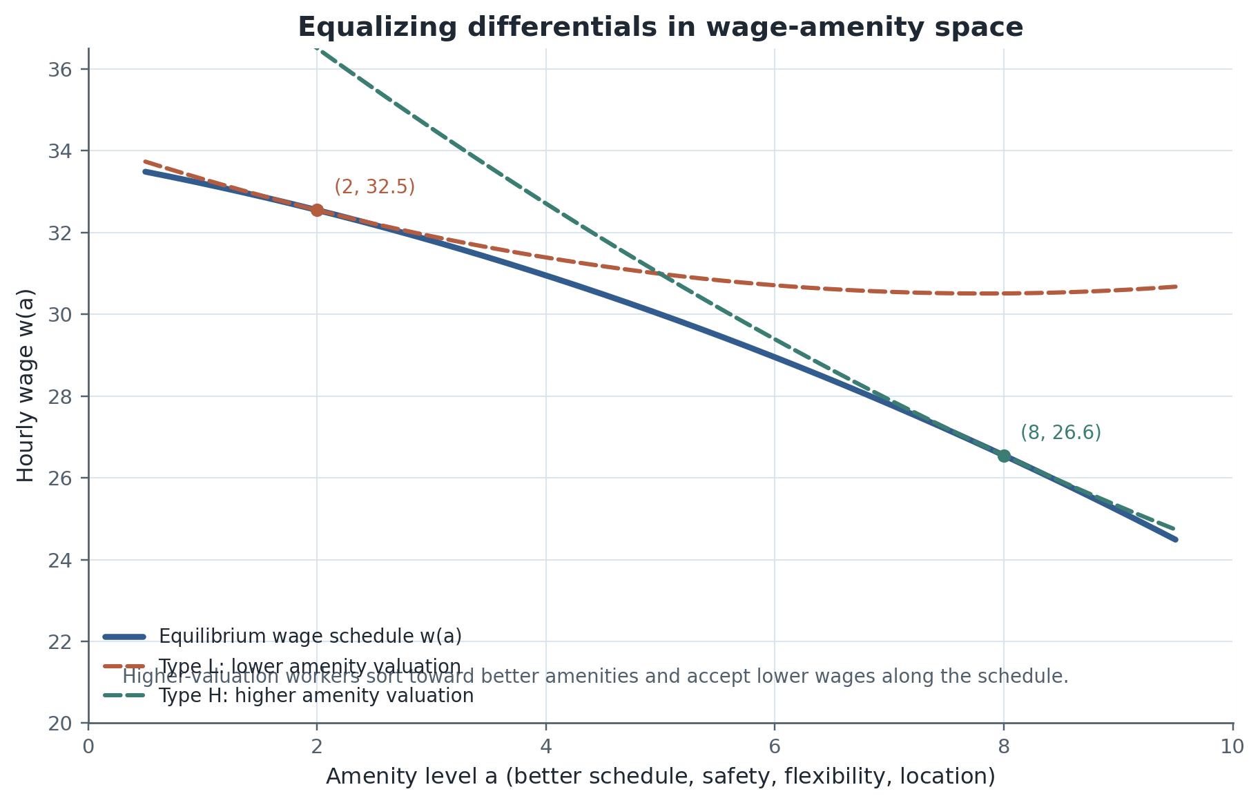
Figure 1:Conceptual hedonic equilibrium in wage-amenity space. The downward-sloping wage schedule shows that better amenities can be purchased with lower wages in equilibrium, while different worker types sort to different tangency points because willingness to pay for amenities is heterogeneous.
Figure Figure 1 is the lecture picture that should anchor the week. Week 6 already hinted that flexibility or predictable schedules can be household inputs when care constraints bind. Week 7 makes that idea market-wide: jobs offering those features can pay differently precisely because workers value them differently.
Field Core
Equalizing differentials and hedonic equilibrium
The canonical benchmark is Rosen’s hedonic model. Workers sort across jobs with different amenities, firms choose which amenity bundles to offer, and competitive equilibrium determines a wage schedule that prices the amenity margin Rosen, 1986. On the worker side, optimal choice along the wage-amenity frontier implies
Equation (2) is the equalizing-differentials condition. The slope of the equilibrium wage schedule equals the worker’s marginal willingness to trade wages for amenities. If is a good, the slope is negative: better jobs can pay less because workers accept part of their compensation in amenity form. If is a bad, the wage schedule slopes upward because unpleasant jobs must compensate workers at the margin.
This condition is powerful precisely because it is equilibrium logic rather than a reduced-form slogan. It says unpleasant jobs need not pay more on average in every sample. They pay more along the margin only after conditioning on the fact that workers with different tastes and outside options sort across jobs. That is why the observed slope in Figure Figure 1 already reflects heterogeneity in both preferences and opportunities.
Firms enter the picture because amenities are costly or productivity-relevant to supply. A reduced-form firm problem is
where is revenue, is the wage required to hire labor under amenity level , and is the direct or indirect cost of offering that amenity bundle. Equation (3) is the shortest route to a serious classroom point: safety equipment, schedule control, remote technology, staffing slack, and reduced monitoring all have firm-side cost or productivity consequences. Amenities are not free gifts. They are jointly determined with wages.
The full hedonic schedule therefore reflects two sets of heterogeneity:
workers differ in , so willingness to pay for the same amenity is not constant;
firms differ in and in the productivity implications of amenities, so the supply side of job quality is heterogeneous as well.
This is why Rosen remains the benchmark, but not a complete empirical design. The theory predicts sorting and endogenous wage-amenity bundles, which means the raw data cannot be read as if jobs were randomly assigned Rosen, 1986Hamermesh, 1999.
Why simple hedonic wage regressions often fail
The fragility of naive hedonic wage regressions is not an embarrassment to the theory. It is mostly a reminder that the theory itself predicts sorting and heterogeneity. Four problems recur.
First, amenities are multidimensional and often poorly measured. Schedule control, advance notice, risk, commute burden, mission, intensity, monitoring, and coworker quality can all matter at once, yet many wage datasets observe only a thin slice of those dimensions. Second, workers sort on unobserved skill, taste, and family constraints. A worker who accepts lower wages for remote work may also differ in home-production demands or outside options, making the cross-sectional wage slope a mixture of preference and selection.
Third, firms bundle amenities. A productive firm may pay high wages, offer remote options, and provide better schedules, which can flatten or even reverse the simple hedonic slope in cross section. Fourth, information frictions, mobility costs, and search frictions break the frictionless equalizing benchmark. Workers may not know the full amenity bundle ex ante, may face costly moves, or may bargain over offers in thin markets. In those environments, observed wages need not reveal the full underlying willingness to pay Hwang et al., 1998Bonhomme & Jolivet, 2009.
The important field-course lesson is therefore asymmetric. A positive wage premium for a bad job attribute is not enough to validate the model, and a zero or wrong-signed premium is not enough to reject it. Empirical failures often reveal multidimensional job quality, heterogeneous preferences, limited mobility, or incomplete information rather than a wholesale collapse of equalizing-differences logic.
Table 1:Week 7 amenity taxonomy
| Amenity class | Typical examples | Why it matters for labor economics | Main empirical challenge |
|---|---|---|---|
| Risks and physical conditions | injury risk, fatality risk, exposure, heat, noise | canonical compensating-differentials object; connects to regulation and VSL | risk mismeasurement, worker selection into risky jobs |
| Schedule and timing | predictable schedule, advance notice, night/weekend work, overtime control | affects labor supply, family compatibility, and stress | schedules are bundled with occupation and firm type |
| Location and commute | remote work, hybrid work, commute time, travel requirements | changes effective value of wages and nonwork time | many datasets omit commute burden or remote options |
| Autonomy and monitoring | worker-controlled flexibility, break autonomy, algorithmic monitoring | changes utility and often productivity | hard to distinguish autonomy from unobserved firm quality |
| Work intensity and pace | staffing ratios, pace pressure, emotional load | affects utility, turnover, and burnout | often poorly measured in wage datasets |
| Prestige and social environment | mission, coworker quality, culture, respect | affects sorting and labor-market welfare | highly subjective and difficult to compare across workers |
Table Table 1 is useful here because it turns “amenities” into a concrete measurement agenda. The empirical challenge is not only that nonwage conditions matter. It is that the relevant conditions are numerous, bundled, and measured with very different quality across datasets.
Empirical strategies: what object is being estimated?
Week 7 evidence is easiest to organize by identifying object rather than chronology.
Hedonic wage regressions estimate a wage-amenity slope in observed cross sections. They are broad in scope and often easy to run, but they are not direct estimates of marginal willingness to pay because worker and firm selection are built into the observed bundles.
Risk-premium studies recover compensation for injury or fatality risk and often map into policy-relevant values of statistical life. They are the classic applied use of equalizing-differentials logic, but risk mismeasurement and selection into dangerous jobs remain central threats Viscusi & Aldy, 2003.
Discrete-choice or conjoint designs estimate willingness to pay for explicit job attributes by varying offers directly. These designs are especially valuable when the researcher wants the valuation of a named amenity such as schedule control or remote work Mas & Pallais, 2017.
Revealed-preference mobility approaches use job-to-job transitions or firm rankings to recover latent job value from actual choices. They move closer to overall job value, but they require richer structure and stronger assumptions about mobility costs, information, or search Bonhomme & Jolivet, 2009Sorkin, 2018.
Broader working-conditions designs estimate how bundles of conditions map into welfare and inequality, bringing job quality back into distributional accounting Maestas et al., 2023.
Table 2:Week 7 empirical design map
| Design | Main identifying object | Strength | Principal threat |
|---|---|---|---|
| Hedonic wage regression | cross-sectional wage-amenity slope | simple and often broad in scope | omitted worker tastes, omitted firm heterogeneity, multidimensional amenities |
| Risk-premium / VSL studies | wage compensation for fatality or injury risk | classic equilibrium application with policy relevance | risk measurement, selection, union/regulation confounds |
| Discrete-choice / conjoint experiment | willingness to pay for explicit attributes | directly estimates marginal valuations of named amenities | external validity, attention, design dependence |
| Revealed-preference worker-flow methods | latent firm/job value from job-to-job choices | uses actual choices rather than stated preferences | requires rich mobility data and stronger structure |
| Working-conditions stated-preference bundle | valuation of broad job-quality bundles | connects amenities to inequality and total compensation | measurement/comparability across job attributes |
Table Table 2 is the organizing device for the empirical part of the lecture. The same observed wage gap can correspond to at least three different estimands: a reduced-form wage-amenity slope, a marginal willingness-to-pay parameter, or a broader revealed-preference ranking over firms or job bundles.
Modern amenities: schedule control, remote work, and job design
Modern empirical work improves on the older hedonic tradition by moving closer to explicit choice objects. A useful discrete-choice representation is
where is a vector of job attributes, such as schedule predictability, remote-work eligibility, injury risk, or worker-controlled flexibility. In this setup, willingness to pay for amenity is recovered as when the wage coefficient is scaled in money units. Equation (4) is one of the most teachable formal objects in the chapter because it turns “amenities matter” into an estimable marginal tradeoff.
Mas and Pallais are the natural Week 7 anchor because they estimate willingness to pay for explicit job attributes rather than inferring it from noisy wage cross sections Mas & Pallais, 2017. Their contribution is not only that workers value flexibility. It is that valuations are large for some attributes and heterogeneous across workers, exactly as Equation (4) predicts. Week 6 matters directly here: a predictable schedule or remote option can be worth more to workers facing childcare or commuting constraints than to otherwise similar workers without those constraints.
Maestas, Mullen, Powell, von Wachter, and Wenger broaden the same logic from a few named attributes to a richer working-conditions bundle Maestas et al., 2023. That move matters because real jobs package amenities jointly. The empirical target is no longer only the value of one isolated schedule feature. It is how total working conditions contribute to compensation, sorting, and inequality.
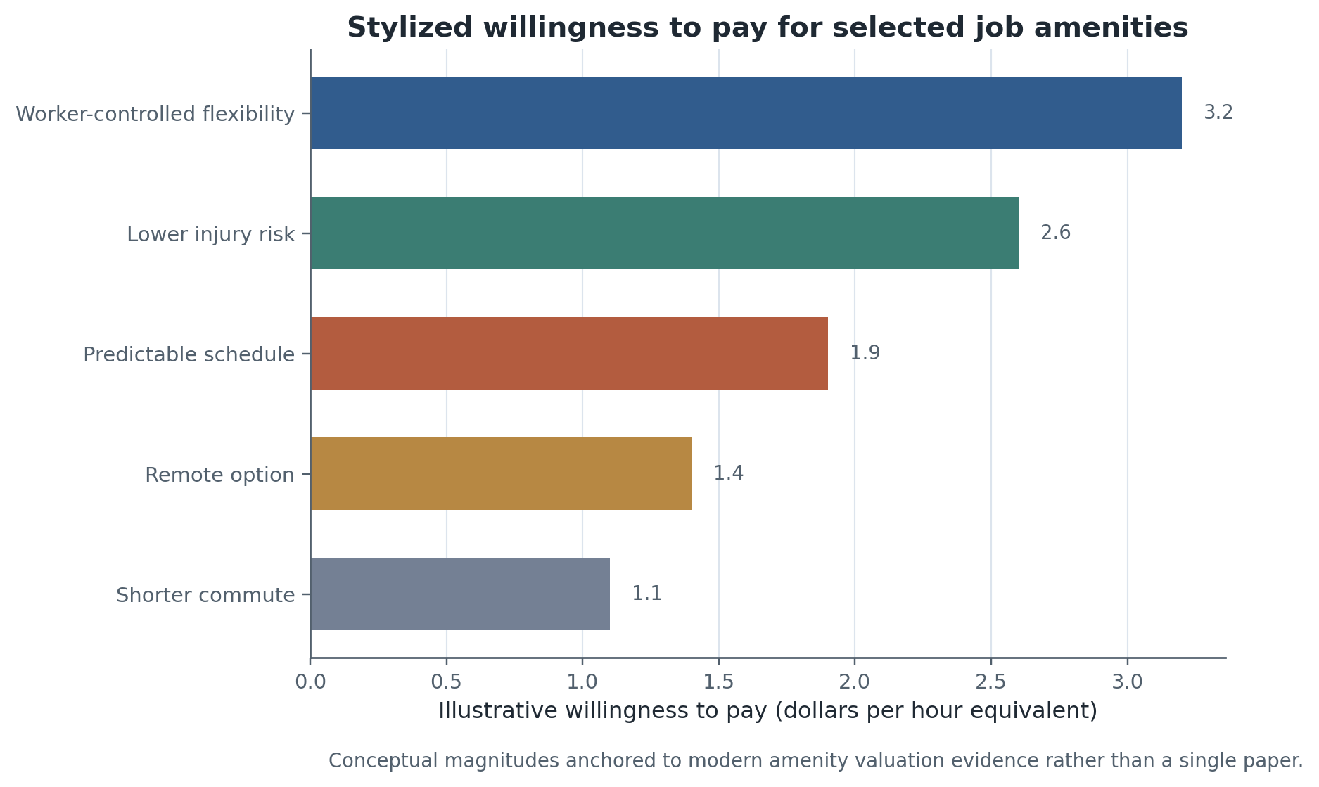
Figure 2:Stylized willingness-to-pay magnitudes for selected job amenities. The figure is conceptual, but it reflects the Week 7 empirical lesson that named amenities such as worker-controlled flexibility, lower risk, predictable schedules, and remote options can command sizable wage-equivalent values.
Figure Figure 2 is helpful because it keeps the lecture from drifting back into vague language about “job quality.” Week 7 is strongest when students see that willingness to pay can be translated into wage-equivalent objects and then compared across amenities, worker types, or family circumstances.
Amenities, sorting, and inequality
Once wages are only one part of compensation, inequality becomes harder and more interesting. Some workers may sort into lower-wage but high-amenity jobs, which means wage inequality can exaggerate welfare inequality. But the opposite can also happen. Workers with strong outside options or access to high-paying firms may receive both high wages and better amenities, in which case wage inequality understates inequality in total job value Card et al., 2018Maestas et al., 2023.
This is the point where Week 7 becomes the bridge into Week 8. Wage dispersion is not automatically the same thing as labor-market inequality because job quality may covary with wages in either direction. A firm wage premium can bundle better schedules, lower risk, career development, and more autonomy. Or some desirable jobs may partly “pay for themselves” through lower wages because workers queue for them. Distributional interpretation therefore depends on how wages and amenities sort jointly across workers and firms.
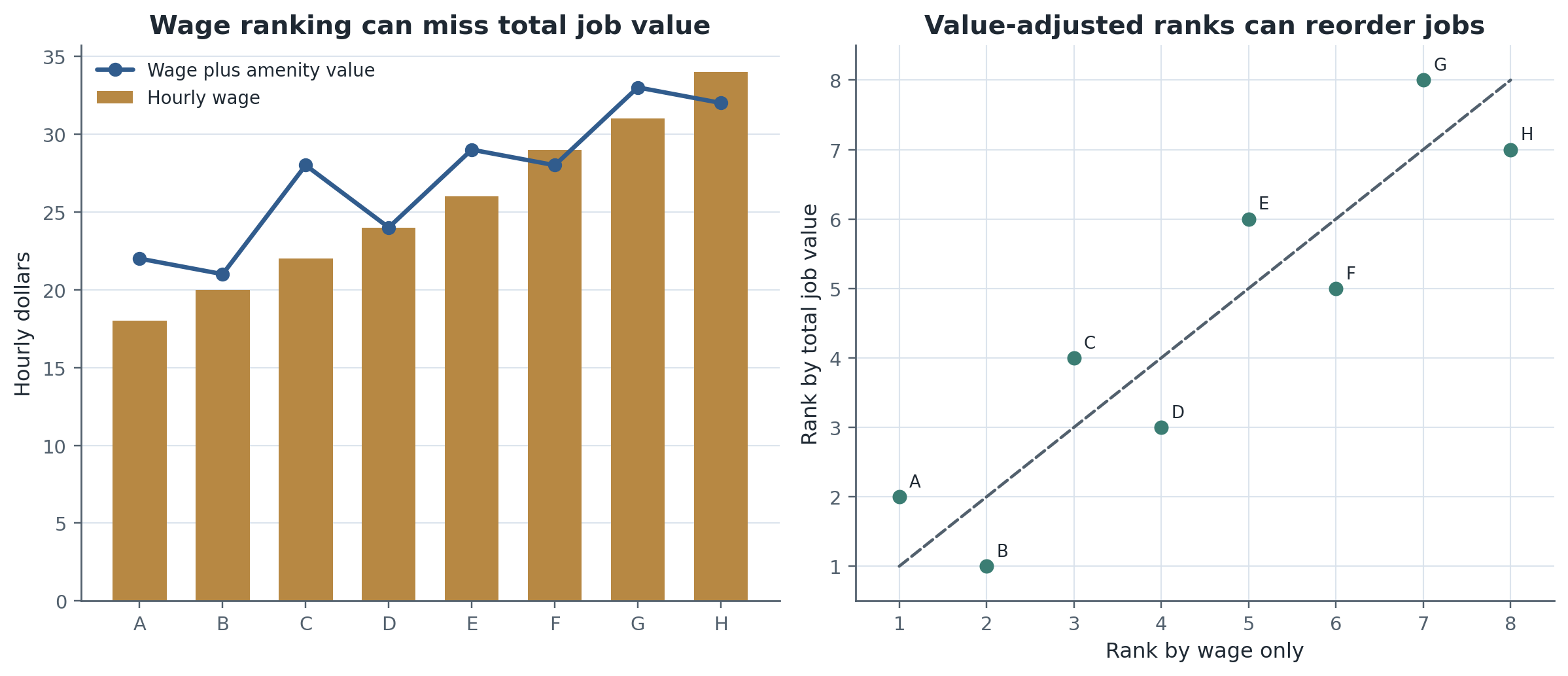
Figure 3:Conceptual comparison of wage-only ranking and total job-value ranking. Some jobs look low in the wage distribution but rank much higher once amenities are valued, while others move downward because unpleasant conditions are omitted when wages alone are used.
Figure Figure 3 is the simplest visual bridge to the next two weeks. Week 8 will ask how to interpret dispersion once jobs differ in total value, and Week 9 will ask whether disadvantaged groups systematically receive worse amenities as well as lower pay. If group differences in job quality are ignored, both inequality and discrimination can be mismeasured.
Why Week 7 is the hinge week
Week 7 changes what counts as compensation. Week 5 showed that observed wages embed productivity, selection, and sorting. Week 6 showed that family structure changes how workers value time and flexibility. Week 7 adds the fact that the same wage can buy very different job bundles. That is why Week 8 should not equate wage dispersion with welfare dispersion, and why Week 9 should not equate discriminatory harm with wage gaps alone. Segmentation can occur in the allocation of schedules, safety, autonomy, and remote work just as much as in posted pay.
Research Lab
The bounded Week 7 lab is built around a Reproduce -> Diagnose -> Transfer path that is fully local and does not require proprietary microdata. The reproduction step uses a synthetic job-choice dataset in the spirit of Mas & Pallais, 2017, where workers choose between offers that differ in wages and explicit amenities. Students recover willingness to pay for schedule predictability, remote work, and worker-controlled flexibility using a discrete-choice approximation that keeps the design transparent.
The diagnostic step asks students to interpret those estimates correctly. A willingness-to-pay parameter is not the same thing as a cross-sectional wage premium, and it is not automatically constant across workers. The lab therefore highlights heterogeneity by showing how care-constrained or commute-burdened workers can place larger value on the same amenity.
The transfer step moves from named attributes to broader working conditions in the spirit of Maestas et al., 2023. Students use a synthetic working-conditions panel to compare wage-only rankings with value-adjusted rankings that incorporate amenity bundles. An optional extension note points to Sorkin, 2018 as the next step from explicit attribute valuation toward revealed-preference rankings over firms and job ladders.
Open research questions should remain visible:
Which amenities are best treated as explicit job attributes and which are better treated as latent firm value?
How much of observed wage inequality disappears or expands once working conditions are monetized?
When do search frictions prevent equalizing differences from arbitraging away bad job conditions?
How should discrimination or segmentation be measured when disadvantaged workers may receive worse job quality as well as lower wages?
Which public datasets best support amenity measurement without collapsing into crude occupation-level proxies?
Methods Box
Week 7 adds one discipline to the wage-setting and household tools from Weeks 5 and 6: never interpret wages without asking what nonwage conditions are bundled with them.
Start with Equation (1) and name the job attribute that enters worker welfare.
Use Equation (2) to distinguish the equilibrium wage slope from raw cross-sectional wage comparisons.
Use Equation (3) to ask which firm costs or productivity channels make an amenity expensive or cheap to supply.
Use Equation (4) to separate a direct willingness-to-pay estimate from a descriptive wage premium.
Before treating a wage gap as an inequality or discrimination fact, ask whether job quality differs systematically across workers, firms, or groups.
Reading Ladder And References
Bridge
Rosen on compensating differentials and hedonic equilibrium Rosen, 1986
Hamermesh on the broader labor-economics importance of demand for job attributes Hamermesh, 1999
Viscusi and Aldy on risk compensation and the value of statistical life Viscusi & Aldy, 2003
Field Core
Hwang, Mortensen, and Reed on compensating wage differentials and labor-market search Hwang et al., 1998
Bonhomme and Jolivet on worker preferences, job heterogeneity, and revealed job values Bonhomme & Jolivet, 2009
Mas and Pallais on willingness to pay for work flexibility and schedule-related amenities Mas & Pallais, 2017
Research Lab
Maestas, Mullen, Powell, von Wachter, and Wenger on working conditions, wages, and inequality Maestas et al., 2023
Sorkin on revealed-preference rankings over firms from worker mobility Sorkin, 2018
Card, Cardoso, Heining, and Kline for the bridge from job bundles and firm heterogeneity to modern inequality accounting Card et al., 2018
Exercises And Discussion Prompts
Use Equation (1) to explain why two workers with the same wage can still have different indirect utility from their jobs.
In Equation (2), when should the wage-amenity slope be negative and when should it be positive? Give one labor-market example of each.
Figure Figure 1 shows two tangency points on the same wage schedule. What worker heterogeneity is needed to rationalize that pattern?
Equation (3) treats amenities as costly or productivity-relevant. Give one example where an amenity raises worker utility but also raises firm productivity, and one where it raises worker utility but raises firm cost.
Use Table Table 2 to compare a hedonic wage regression with a discrete-choice design. Which one is closer to a direct willingness-to-pay object, and what does it sacrifice?
Figure Figure 3 shows rank reversals once amenities are monetized. Under what sorting pattern would accounting for amenities reduce measured inequality, and under what pattern would it increase it?
Why does Week 7 imply that Week 9 discrimination should measure access to safe, flexible, predictable, or remote jobs rather than focusing only on wages?
Reproducibility And Code Lab Note
The Week 7 lab is organized around a bounded Reproduce -> Diagnose -> Transfer path that runs fully locally. Students reproduce a synthetic discrete-choice amenity valuation exercise in the spirit of Mas & Pallais, 2017, diagnose what a willingness-to-pay estimate does and does not identify relative to a hedonic wage slope, and then transfer the workflow to a synthetic working-conditions and inequality exercise in the spirit of Maestas et al., 2023. An optional extension note points to worker-flow revealed preference in Sorkin, 2018. The bounded workflow is documented in lab.md.
Slide Companion Note
The Week 7 deck should isolate the move from wages to job bundles, the Rosen hedonic benchmark, why hedonic regressions often fail, modern willingness-to-pay evidence, the amenity taxonomy and empirical design tables, and the bridge from amenities to Week 8 inequality and Week 9 discrimination or segmentation rather than reproducing the full chapter. The canonical source is 07
Bridge Forward
Use this closing bridge to carry the module’s labor object, mechanism, and evidence into the next course step or research-design exercise.
- Rosen, S. (1986). The Theory of Equalizing Differences. In O. C. Ashenfelter & R. Layard (Eds.), Handbook of Labor Economics (Vol. 1, pp. 641–692). Elsevier. 10.1016/S1573-4463(86)01015-5
- Mas, A., & Pallais, A. (2017). Valuing Alternative Work Arrangements. American Economic Review, 107(12), 3722–3759. 10.1257/aer.20161500
- Maestas, N., Mullen, K. J., Powell, D., von Wachter, T., & Wenger, J. B. (2023). The Value of Working Conditions in the United States and the Implications for the Structure of Wages. American Economic Review, 113(7), 2007–2047. 10.1257/aer.20190846
- Hamermesh, D. S. (1999). Changing Inequality in Markets for Workplace Amenities. Quarterly Journal of Economics, 114(4), 1085–1123. 10.1162/003355399556250
- Viscusi, W. K., & Aldy, J. E. (2003). The Value of a Statistical Life: A Critical Review of Market Estimates throughout the World. Journal of Risk and Uncertainty, 27(1), 5–76. 10.1023/A:1025598106257
- Hwang, H., Mortensen, D. T., & Reed, W. R. (1998). Hedonic Wages and Labor Market Search. Journal of Labor Economics, 16(4), 815–847. 10.1086/209907
- Bonhomme, S., & Jolivet, G. (2009). The Pervasive Absence of Compensating Differentials. Journal of Applied Econometrics, 24(5), 763–795. 10.1002/jae.1074
- Sorkin, I. (2018). Ranking Firms Using Revealed Preference. Quarterly Journal of Economics, 133(3), 1331–1393. 10.1093/qje/qjy001
- Card, D., Cardoso, A. R., Heining, J., & Kline, P. (2018). Firms and Labor Market Inequality: Evidence and Some Theory. Journal of Labor Economics, 36(S1), S13–S70. 10.1086/694153