Static Labor Supply
Learning Objectives
By the end of Week 2, students should be able to:
write down the static labor-supply problem and interpret its main comparative statics;
separate intensive-margin hours responses from extensive-margin participation responses in a policy-relevant way;
analyze piecewise-linear budget sets created by taxes and transfers;
explain why fixed work costs and benefit loss make nonparticipation a first-order object rather than a corner case to ignore;
interpret the EITC evidence as evidence about margins, information, and schedule geometry rather than as a single elasticity estimate;
connect the static benchmark back to Week 1 measurement objects and forward to Weeks 3, 11, and 12.
Opening Orientation
The economic question for the week is direct: once wages, taxes, transfers, and work costs are taken seriously, how do workers choose whether and how much to work in a static environment?
Bridge
Week 1 gave us the empirical objects: participation, hours, earnings, and tax-adjusted incentives. Week 2 gives the first formal benchmark for organizing those objects. The static labor-supply model remains indispensable because it is the cleanest map from a policy wedge into behavioral predictions. When the after-tax return to work changes, the benchmark tells us where to look first: entry into work, hours conditional on work, or both.
The benchmark is intentionally narrow. It takes wages and the tax-transfer schedule as given. It abstracts from savings, learning, and dynamic adjustment. That narrowness is a feature before it becomes a limitation. It lets us say clearly what the theory predicts before later weeks add intertemporal substitution, persistence, and informational frictions. In that sense, static labor supply is the worker-side analogue of Week 1 measurement discipline: a minimal object that later extensions must respect rather than bypass.
The static benchmark
The canonical static problem is
Equation (1) treats hours as the choice variable, nonlabor income as given, and as the full tax-transfer schedule rather than a single linear tax. The object of interest is already policy-facing: the return to an additional hour depends on where the worker sits on the schedule.
If the worker is interior, the key optimality condition is
Equation (2) says that the marginal rate of substitution between leisure and consumption must equal the net-of-tax wage. This is the static benchmark that underlies most comparative statics in public economics and labor supply. A tax change matters through the net reward to an extra unit of work, but the size and sign of the total response still depend on income effects, preference heterogeneity, and where the worker is relative to participation.
Intensive versus extensive margins
The static model becomes policy-relevant only once we separate two margins. The intensive margin asks how hours change among those already working. The extensive margin asks whether work occurs at all. Many empirical debates that look like disagreements about “the labor-supply elasticity” are really disagreements about which of those two objects is moving, for whom, and under which policy environment Blundell & MaCurdy, 1999Hausman, 1985.
That is why nonparticipation cannot be handled as a cosmetic corner solution. With a fixed work cost , the participation condition is
Equation (3) makes the extensive margin threshold-based. A worker may face a modest hours response conditional on employment and still show a large participation response if policy changes move the value of work across the threshold created by childcare costs, commuting time, benefit loss, or administrative burden. That is the first reason the EITC literature became central to labor supply: it shifted the empirical center of gravity toward participation responses among populations close to the work/nonwork boundary.
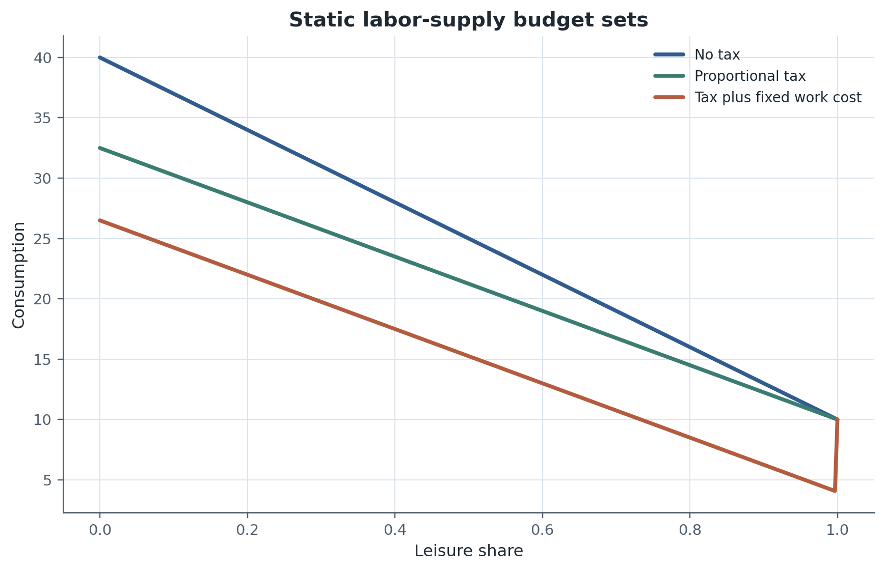
Figure 1:Stylized budget sets for the static labor-supply problem. The figure contrasts a no-tax benchmark, a proportional tax, and a fixed-cost environment that introduces a participation wedge. The same wage change can therefore operate differently near the work/nonwork threshold than far from it.
Figure Figure 1 is useful precisely because it puts Equations (1) through (3) on the same geometry. Proportional taxes flatten the line and mainly speak to the intensive condition in Equation (2). Fixed work costs create a discrete gap between nonwork and work, which is why the extensive margin often dominates for groups with low baseline attachment or high effective work costs.
Field Core
Taxes, transfers, and nonlinear budget sets
Real policy environments rarely offer the linear budget line that makes blackboard comparative statics feel clean. Taxes and transfers generate piecewise-linear schedules with kinks, plateaus, and phase-outs. Means-tested benefits can lower the effective return to earnings in one region and raise it in another. A single policy therefore need not move all workers in the same direction even when it applies to all of them.
The EITC is the most useful Week 2 bridge because its geometry makes this point immediately. In the phase-in region, earnings are subsidized and entry into work becomes more attractive. On the plateau, marginal incentives look different from average incentives. In the phase-out region, effective marginal tax rates rise, so the relevant labor-supply question becomes whether workers reduce hours, remain unchanged because of frictions or salience limits, or adjust along other margins.
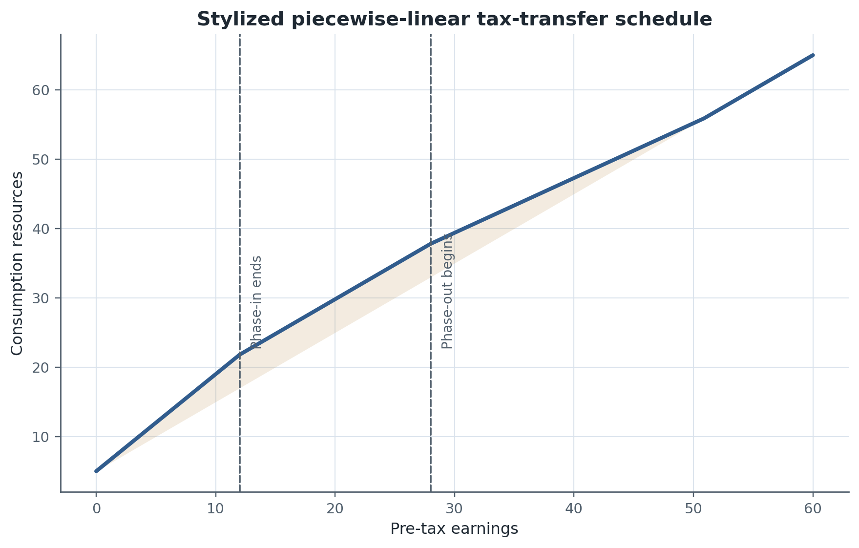
Figure 2:Stylized piecewise-linear tax-transfer schedule with phase-in, plateau, and phase-out regions. The point is conceptual rather than calendar-specific: static labor supply under public policy is usually a problem with local slopes and threshold regions, not a single linear wage.
Figure Figure 2 shows why the textbook linear model is not enough for policy interpretation. Once the slope changes across regions, the relevant treatment is local to the worker’s position on the schedule. That is the geometric intuition behind kink-based evidence, bunching evidence, and heterogeneous EITC responses.
Table 1:Elasticity taxonomy for static labor supply
| Elasticity object | Main margin | Common empirical design | Main interpretation risk |
|---|---|---|---|
| Uncompensated intensive-margin elasticity | Hours conditional on work | Tax reforms, wage variation, panel estimates | Mixes income and substitution effects |
| Compensated intensive-margin elasticity | Hours conditional on work | Structural or sufficient-statistics adjustments | Hard to recover without additional assumptions |
| Extensive-margin participation elasticity | Work / nonwork choice | EITC reforms, welfare reforms, threshold variation | Sensitive to fixed costs, childcare, and benefit loss |
| Taxable-income elasticity | Reported earnings / taxable income | Kink or bunching designs | May reflect evasion, avoidance, or timing rather than real labor supply |
| Macro labor-supply elasticity | Aggregate hours / participation | Cross-regime comparisons, long-run reforms | Captures adjustment, equilibrium, and institution responses |
Table Table 1 is a better organizer of the evidence than a list of headline numbers. It separates compensated from uncompensated intensive responses, distinguishes participation from hours, and warns that taxable-income elasticities need not be real labor-supply elasticities. This is where Chetty’s synthesis matters most: different empirical designs recover different objects when adjustment costs and optimization frictions prevent all margins from moving freely Chetty, 2012.
Table 2:Policy instruments and labor-supply margins
| Policy instrument | Expected primary margin | Why | Major caveat |
|---|---|---|---|
| Proportional income-tax change | Intensive margin | Changes net-of-tax reward to an extra hour | Can miss participation and avoidance channels |
| EITC expansion | Extensive margin in many populations | Increases payoff to entering work in the phase-in region | Intensive responses differ across schedule regions |
| Childcare subsidy | Extensive margin plus hours | Lowers effective fixed cost of work | Effects may depend on household bargaining and local supply |
| Work requirement / welfare reform | Participation | Changes outside option and eligibility rules | Often bundled with multiple policy changes |
| Payroll-tax change | Hours, employment, or wages depending on incidence | Changes labor cost or take-home pay | Incidence may not fall on workers one-for-one |
Table Table 2 turns that taxonomy into policy language. An EITC expansion is not merely “a tax cut.” For many low-income single parents, it loads first on participation because it changes the value of entering work. A childcare subsidy can operate through both participation and hours because it directly lowers the fixed cost in Equation (3). A payroll-tax change may affect hours, employment, or wages depending on incidence. The policy lesson is that labor-supply debates are really about which margin the instrument is built to move.
What empirical elasticities mean
The classic static model gives clean comparative statics, but empirical elasticities are recovered from environments in which workers may not know the schedule perfectly, may adjust with delay, or may face discrete constraints on hours. That is why the literature contains what at first looks like disagreement. A micro estimate from a tax reform, a bunching estimate around a kink, and an aggregate cross-regime comparison are not automatically measuring the same object Blundell & MaCurdy, 1999Chetty, 2012.
Three distinctions keep the empirical interpretation disciplined.
First, uncompensated and compensated intensive elasticities answer different questions. The uncompensated object mixes substitution and income effects; the compensated object strips away the income channel but is harder to recover without stronger structure. Second, participation elasticities are inherently threshold-based, so they are sensitive to fixed costs, benefit cliffs, and household constraints. Third, taxable-income responses may reflect reporting, avoidance, timing, or real effort. In a nonlinear schedule, all three distinctions matter simultaneously.
Chetty’s contribution is not merely to split the difference across papers. It is to explain why some environments generate small observed intensive responses even when underlying long-run labor-supply objects need not be tiny. Optimization frictions, salience limits, and adjustment costs can compress observed short-run responses, especially where the return to fine-tuning hours is modest Chetty, 2012. That interpretation is especially useful for connecting bunching evidence to the broader labor-supply literature rather than treating it as a separate tax niche.
The EITC as the applied bridge
The EITC literature is the week’s central empirical application because it links schedule geometry, participation, and policy interpretation in a single setting. Eissa and Liebman show that the 1986 expansion generated substantial participation responses among single mothers, with much weaker evidence of large hours changes conditional on work Eissa & Liebman, 1996. The key lesson is not simply that labor supply exists; it is that the extensive margin can be the first-order policy channel when the schedule increases the payoff to entering employment.
Eissa and Hoynes extend the perspective to married couples and show why household context matters for the same policy Eissa & Hoynes, 2004. An EITC expansion can raise incentives for one spouse while reducing them for the secondary earner, depending on where family earnings place the household on the schedule. The static model therefore needs a household interpretation even before we reach the family module later in the semester.
The broader review in Eissa and Hoynes organizes the lesson cleanly: empirical labor-supply responses to the EITC are heterogeneous because the policy changes average and marginal incentives differently across families and across regions of the schedule Eissa & Hoynes, 2006. That is exactly the kind of policy-to-margin mapping summarized in Table Table 2.
Saez adds a complementary perspective by studying bunching at kink points in the tax schedule Saez, 2010. Bunching evidence is attractive because Figure Figure 2 implies that local slope changes create local incentives to concentrate earnings near a kink. But the interpretation is subtle. Some taxpayers bunch strongly and others do not; some responses may reflect reporting or adjustment of taxable income rather than hours; and the amount of bunching can be dampened when the schedule is poorly understood or costly to optimize around.
Chetty, Friedman, and Saez sharpen that last point by showing that local knowledge and information frictions shape observed EITC responses Chetty et al., 2013. Their lesson is not that the static benchmark is wrong. It is that the benchmark delivers the right comparative statics only once we ask what workers know about the schedule and whether they can act on that knowledge. That is the bridge to Week 12, where information, attention, and behavioral responses stop being an add-on and become part of the model itself.
Research Lab
The frontier issue is not whether the static model should be discarded. It is which empirical object remains informative once the environment includes nonlinear schedules, fixed costs, limited salience, and household interactions. One open research direction asks how far extensive-margin elasticities travel across institutional settings. A participation response to the EITC among single mothers in the 1990s is not automatically the right object for forecasting responses to childcare subsidies, payroll-tax changes, or reforms in countries with different transfer systems.
Another frontier issue is measurement of the relevant response variable. Bunching in taxable income is a sharp design, but taxable income can move because reported earnings move, timing shifts, deductions change, or formal labor supply changes. That makes Week 2 a natural bridge between labor economics and public finance rather than a purely worker-choice chapter.
The research payoff from the week comes from treating the benchmark as indispensable and incomplete at the same time. Week 3 will add intertemporal substitution and lifecycle adjustment. Week 11 will revisit the same margins in a broader worker-policy evaluation framework. Week 12 will ask how informational and behavioral frictions change both elasticities and welfare interpretation. Week 2 matters because those later modules only make sense if the static benchmark is already clear.
Methods Box
Week 2 uses a simple translation rule from theory to empirical design.
Write the choice problem and identify whether the policy shifts the average return to work, the marginal return, or both.
Ask whether the relevant outcome is participation, hours conditional on work, earnings, or taxable income.
Check whether the budget set is linear, piecewise linear, kinked, or nonconvex.
Decide whether the design identifies a local response near a threshold or a broader behavioral object.
Interpret the estimate in light of information, adjustment, and reporting frictions.
The point is to keep Equations (1), (2), and (3) tied to data rather than leaving them as pure diagrammatic intuition.
Reading Ladder And References
Bridge
Blundell and MaCurdy on the static benchmark and how labor-supply objects are defined Blundell & MaCurdy, 1999
Hausman on taxes, nonlinear budget sets, and the public-finance interpretation of labor supply Hausman, 1985
Field Core
Eissa and Liebman on single-mother participation responses to the EITC Eissa & Liebman, 1996
Eissa and Hoynes on married-couple labor-supply responses under the EITC Eissa & Hoynes, 2004
Eissa and Hoynes on broader lessons from the EITC literature Eissa & Hoynes, 2006
Chetty on labor-supply elasticities with optimization frictions Chetty, 2012
Research Lab
Saez on bunching at kink points and the interpretation of local nonlinear-budget responses Saez, 2010
Chetty, Friedman, and Saez on knowledge frictions and EITC responses Chetty et al., 2013
Optional structural extensions on work costs and piecewise-linear budgets Heim & Meyer, 2004Fullerton & Gan, 2004
Exercises And Discussion Prompts
Use Equations (2) and (3) to explain why the same policy can generate small hours responses but large participation responses.
In Figure Figure 2, which region of the schedule is most naturally associated with entry into work, and which region is most naturally associated with hours adjustment? Defend your answer.
Why is the taxable-income elasticity in Table Table 1 not automatically a labor-supply elasticity?
Eissa and Hoynes show that married-couple responses need not match single-mother responses. Which object in the static model is doing the work?
If bunching is weak in a setting with strong formal incentives, what are the leading interpretations before concluding that labor supply is inelastic?
Reproducibility And Code Lab Note
The Week 2 lab is built around a bounded teaching path for Saez, 2010. Students reproduce a stylized bunching figure using the local synthetic dataset and the Python scripts in labs/02-static-labor-supply/src/, then transfer the same workflow to an alternative subgroup or bin-width choice. The full official AEA replication package remains the intellectual benchmark, but the bounded path deliberately avoids requiring the full external package for the smoke test. The lab note at lab.md documents the exact external files still needed for a closer reproduction using the official materials.
Slide Companion Note
The slide deck should isolate the benchmark problem, the margin decomposition, the nonlinear-budget geometry, and the empirical EITC lessons without turning the chapter into text-heavy slides. The deck at 02
Bridge Forward
Use this closing bridge to carry the module’s labor object, mechanism, and evidence into the next course step or research-design exercise.
- Blundell, R., & MaCurdy, T. (1999). Labor Supply: A Review of Alternative Approaches. In O. Ashenfelter & D. Card (Eds.), Handbook of Labor Economics (Vol. 3A, pp. 1559–1695). Elsevier. 10.1016/S1573-4463(99)03008-4
- Hausman, J. A. (1985). Taxes and Labor Supply. Handbook of Public Economics.
- Chetty, R. (2012). Bounds on Elasticities with Optimization Frictions: A Synthesis of Micro and Macro Evidence on Labor Supply. Econometrica, 80(3), 969–1018. 10.3982/ECTA9046
- Eissa, N., & Liebman, J. B. (1996). Labor Supply Response to the Earned Income Tax Credit. The Quarterly Journal of Economics, 111(2), 605–637. 10.2307/2946689
- Eissa, N., & Hoynes, H. W. (2004). Taxes and the Labor Market Participation of Married Couples: The Earned Income Tax Credit. Journal of Public Economics, 88(9–10), 1931–1958. 10.1016/S0047-2727(03)00041-5
- Eissa, N., & Hoynes, H. W. (2006). Behavioral Responses to Taxes: Lessons from the EITC and Labor Supply. Tax Policy and the Economy, 20, 73–110. 10.1086/tpe.20.20061838
- Saez, E. (2010). Do Taxpayers Bunch at Kink Points? American Economic Journal: Economic Policy, 2(3), 180–212. 10.1257/pol.2.3.180
- Chetty, R., Friedman, J. N., & Saez, E. (2013). Using Differences in Knowledge across Neighborhoods to Uncover the Impacts of the EITC on Earnings. American Economic Review, 103(7), 2683–2721. 10.1257/aer.103.7.2683
- Heim, B. T., & Meyer, B. D. (2004). Structural Labor Supply Models when Budget Constraints are Nonlinear. NBER Working Paper, w11176.
- Fullerton, D., & Gan, L. (2004). A Simulation-Based Difference-in-Difference Estimator for Evaluating the Effect of a Tax Reform on Labor Supply and Welfare. Journal of Public Economics, 88(3–4), 623–650. 10.1016/S0047-2727(02)00130-6